Chapter 6 PCA (mathematical details)
Welcome to the last section of this chapter. We are going to talk a bit about the mathematical details of PCA. It’s important that it’s not necessary to understand the mathematical details of PCA in order to effectively apply this amazing method to your data. One can easily skip this section without having any problems when it comes to the application. So feel free to skip this if you find it difficult to follow!
6.1 Summary of the previous chapter
Since the beginning of this chapter, we have been talking about variance as a measure of variability in our data. We also talked a bit about covariance as a measure of concordance or redundancy in our data (or even total variance). We saw that working with high-dimensional data is challenging and PCA can help us summarize these dimensions (e.g. genes) into a set of new variables (scores/components) so that we see the pattern of data spread. The new dimensions were promised to be orthogonal (no covariance) and sorted so that the variance of the first variable is always higher than the second one and so on. We are now ready to see how PCA does this amazing calculation.
6.2 Foundations
In order to understand the math behind PCA, we need to agree on a set of definitions.
For example in our data, we have n=45101 that is equal to the number of genes we have measured, meaning that space our data has 45101 dimensions. You can think about the extent of these dimensions to be all possible expressions of each gene. For example, if we only have two genes in our data, we have \({\rm I\!R}^2\) giving us a 2-dimensional space. The size of this space starts from the lowest possible value for the expression of the genes to the highest possible value. The exact measured expression of each gene gives us the location of our observation in the space.
# Select variable
var1<-18924
var3<-18505
# plot the data for variable 1
plot(data[,c(var1,var3)],xlab = "Variable 1",ylab = "Variable 2",
     ylim = c(0,15),xlim=c(0,20))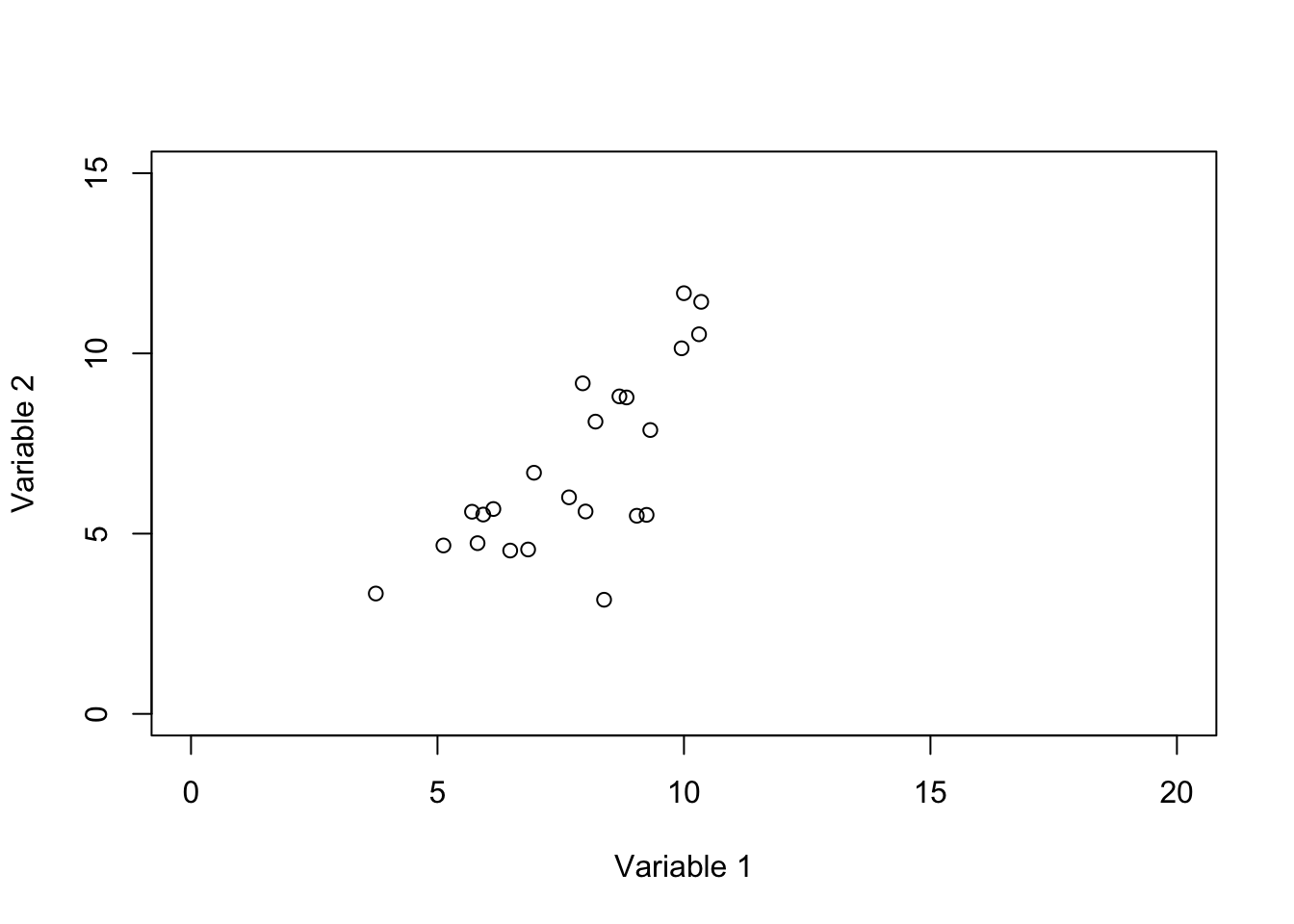
Figure 6.1: Plot of two genes showing the space defined by these two variables
In Figure 6.1 we show two variables. the value of variable 1 starts from 0 and goes all the way to 20 whereas the value of variable 2 starts from 0 and goes to 15. So to put it in context, our space is defined by these variables and their possible values. Our observations (e.g. samples) are just some points or locations in that space. However, for simplicity, we limit the extent of the values to the ones that we observed in our data and not all possible values of variables 1 and 2.
Another way of thinking about space is to imagine outer space which more or less defines what exists in the universe and planets, stars, and in general celestial bodies are located somewhere in space.
knitr::include_graphics(rep('https://www.jpl.nasa.gov/spaceimages/images/wallpaper/PIA22564-640x350.jpg'))
# plot the data for variable 1
plot(c(-2,2),c(-2,2),xlab = "",ylab = "",
 axes = F,type = "n")

# plot the axis
axis(1,cex=4,pos = c(0,0) )
axis(2,cex=4,pos = c(0,0) )

# plot arrow and text
arrows(1,1,0,0)
text(c(1.1),label = "Origin (0,0)")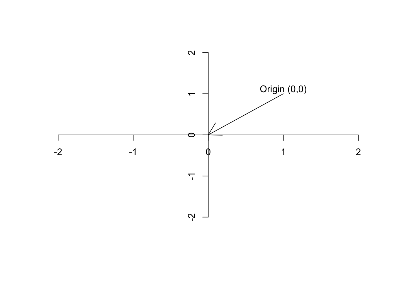
Figure 6.2: Plot of the origin
Definition 6.4 (Vector) A vector is basically just a list of numbers, showing a location of a point in space. We like to show the vectors by their name and a small arrow on top of them (\(\vec{a}\)). For example, if we say \(\vec{a}=[5,13]\), it means we are referring to a point in space where the value for the first axis is 2 and the second axis is 13. It’s often nice to show the vector with an arrow starting from the origin and finishing exactly at that point.
# plot the data for variable 1
plot(c(-20,20),c(-20,20),xlab = "",ylab = "",
 axes = F,type = "n")

# plot the point
points(5,13)
# plot the axis
axis(1,cex=4,pos = c(0,0) )
title(xlab="x", line=-10, cex.lab=1.2,adj=1)
axis(2,cex=4,pos = c(0,0) )
title(ylab="y", line=-17, cex.lab=1.2,adj=1)
# plot arrow and text
arrows(0,0,5,13)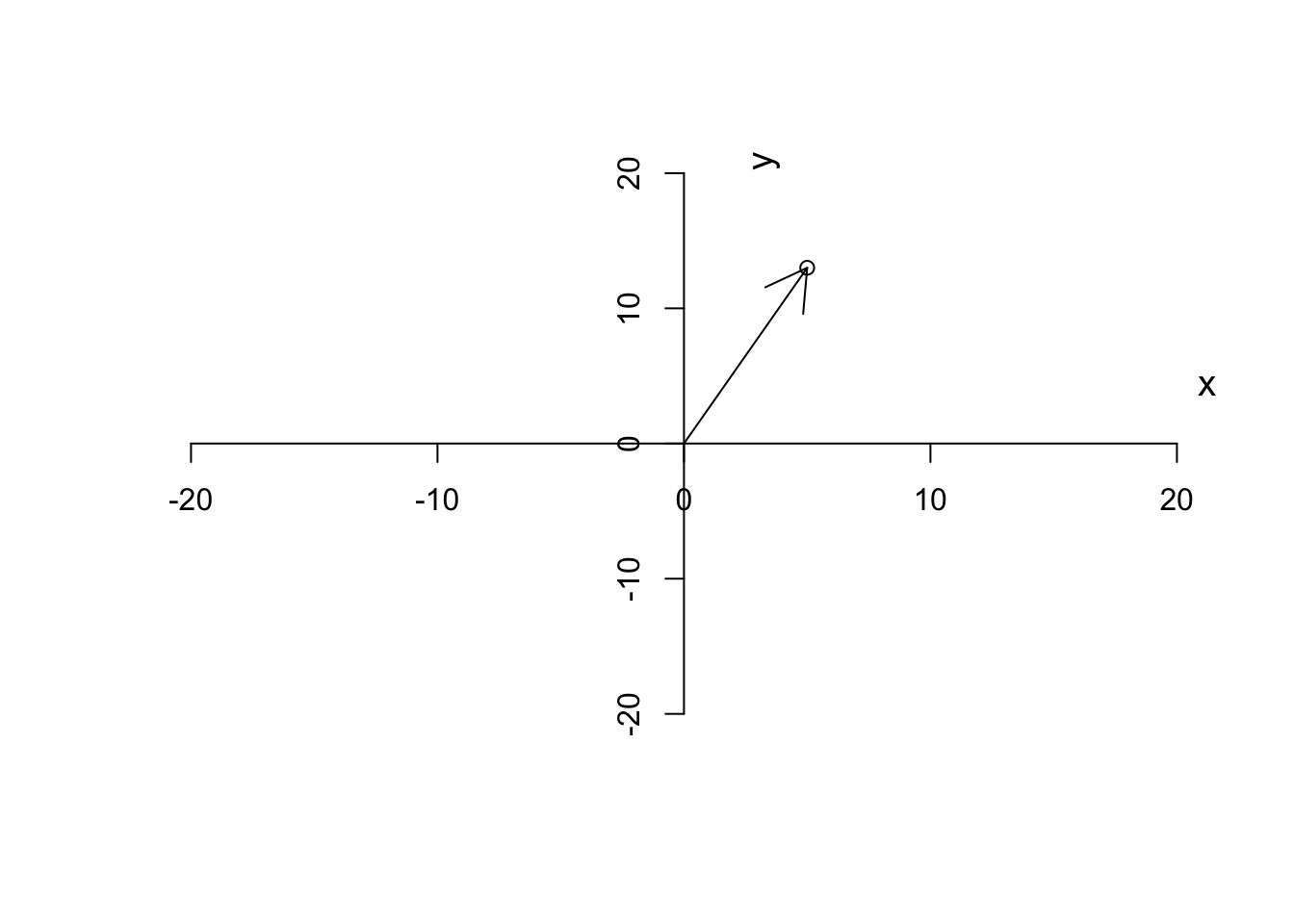
Figure 6.3: Plotting a vector
As we said, we like to put our starting point at \((0,0)\). Given this, we can also think about a vector, has magnitude (length of the arrow starting from the origin or distance to the origin), and also the direction to which the arrow is pointing. So in our case, we have a vector that is defined by going to the right along the \(x\) axis (red arrow in Figure 6.4) until reaching point 3 and the start going up along the \(y\) axis (blue arrow in Figure 6.4) to reach the final point.
# plot the data for variable 1
plot(c(-20,20),c(-20,20),xlab = "",ylab = "",
 axes = F,type = "n")

# plot the point
points(5,13)
# plot the axis
axis(1,cex=4,pos = c(0,0) )
title(xlab="x", line=-10, cex.lab=1.2,adj=1)
axis(2,cex=4,pos = c(0,0) )
title(ylab="y", line=-16, cex.lab=1.2,adj=1)
# plot arrow and text
arrows(0,0,5,13)
arrows(0,0,5,0,col="Red",lty = "dashed")
arrows(5,0,5,13,col="blue",lty = "dashed")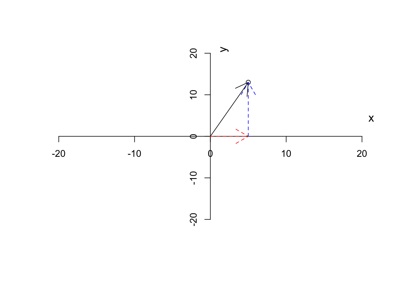
Figure 6.4: Plotting a vector and the steps
The magnitude of a vector is calculated by:
\[\|\vec{a}\|=\sqrt{x^2+y^2}\] Where \(x\) and \(y\) are the first and the second element of the vector. So in our case that is equal to \(\|\vec{a}\|=\sqrt{5^2+13^2}=13.93\).
We normally like to measure the direction of a vector based on the angle it makes with the \(x\) axis.
\[\theta=\tan^{-1}\frac{x}{y}\] This thing can easily be calculated in R for example by
atan(y/x)# plot the data for variable 1
plot(c(-20,20),c(-20,20),xlab = "",ylab = "",
axes = F,type = "n")
# plot the point
points(5,13)
# plot the axis
axis(1,cex=4,pos = c(0,0) )
title(xlab="x", line=-10, cex.lab=1.2,adj=1)
axis(2,cex=4,pos = c(0,0) )
title(ylab="y", line=-16, cex.lab=1.2,adj=1)
# plot arrow and text
arrows(0,0,5,13)
# draw arc
plotrix::draw.arc(0,0,3,angle2=1)
# write text
text(1,1,"1.2",cex=0.7)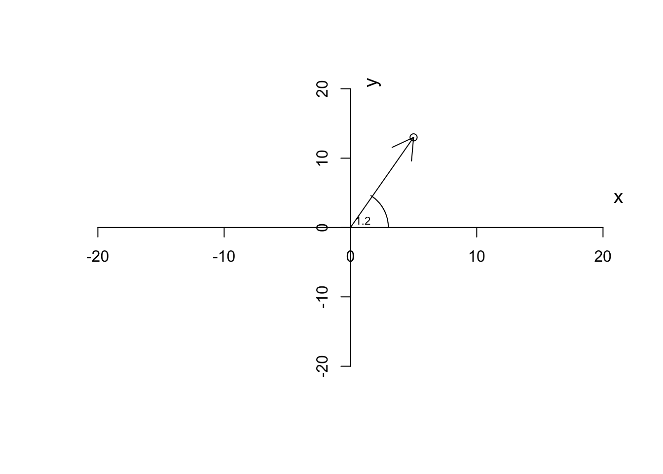
Figure 6.5: Plotting a vector and the steps
So by now, we have the magnitude and direction of a vector. A vector also has a span. A span of a vector is a line resulted in stretching the vector from both ends to infinity.
# plot the data for variable 1
plot(c(-20,20),c(-20,20),xlab = "",ylab = "",
 axes = F,type = "n")

segments(-500,-1300,500,1300,col = "red",lty = "dashed")
text(13,20,"span of the vector",col="red")
# plot the point
points(5,13)
# plot the axis
axis(1,cex=4,pos = c(0,0) )
title(xlab="x", line=-10, cex.lab=1.2,adj=1)
axis(2,cex=4,pos = c(0,0) )
title(ylab="y", line=-16, cex.lab=1.2,adj=1)
# plot arrow and text
arrows(0,0,5,13)
# draw circle
plotrix::draw.arc(0,0,3,angle2=1)

text(1,1,"1.2",cex=0.7)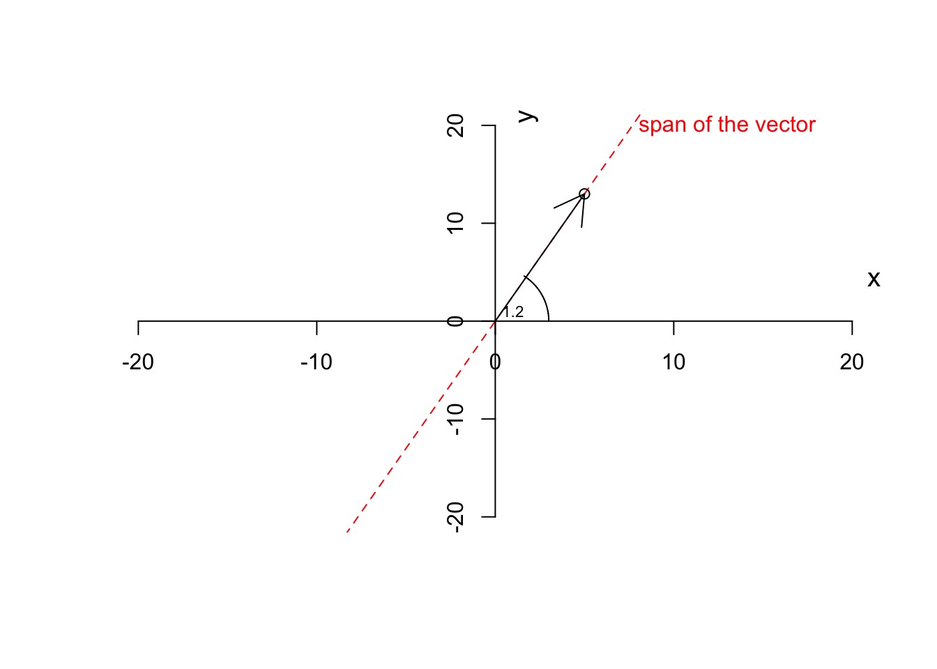
Figure 6.6: Plotting a vector and the steps
Now we can go ahead and define some preliminary operations on the vector.
6.3 Operations on vectors
Definition 6.5 (Scalar multiplication) If we multiply a vector by a scalar (a number) other than one (1), the resulting vector will change magnitude by not direction. However, a vector might flip (pointing to the opposite direction) but it will NEVER change the direction of its span.
When we multiply a scalar to a vector, we take each element of the vector (e.g. \(x\) and \(y\)) and we multiply each of them by that scalar
\[\vec{a} \times j=[x\times j,y\times j]\]
where \(\vec{a}\) is a vector and \(j\) is a scalar.For example if we take our vector \(\vec{a}=[5,13]\) and multiply by \(1.5\) the results will be \([5 \times 1.5, 13 \times 1.5]=[7.5,19.5]\):
# plot the data for variable 1
plot(c(-20,20),c(-20,20),xlab = "",ylab = "",
 axes = F,type = "n")

segments(-500,-1300,500,1300,col = "red",lty = "dashed")
text(13,20,"span of the vector",col="red")

# plot the axis
axis(1,cex=4,pos = c(0,0) )
title(xlab="x", line=-10, cex.lab=1.2,adj=1)
axis(2,cex=4,pos = c(0,0) )
title(ylab="y", line=-16, cex.lab=1.2,adj=1)
# plot arrow and text

arrows(0,0,5*1.5,13*1.5,col="green")
arrows(0,0,5,13)

# draw circle
plotrix::draw.arc(0,0,3,angle2=1)

text(1,1,"1.2",cex=0.7)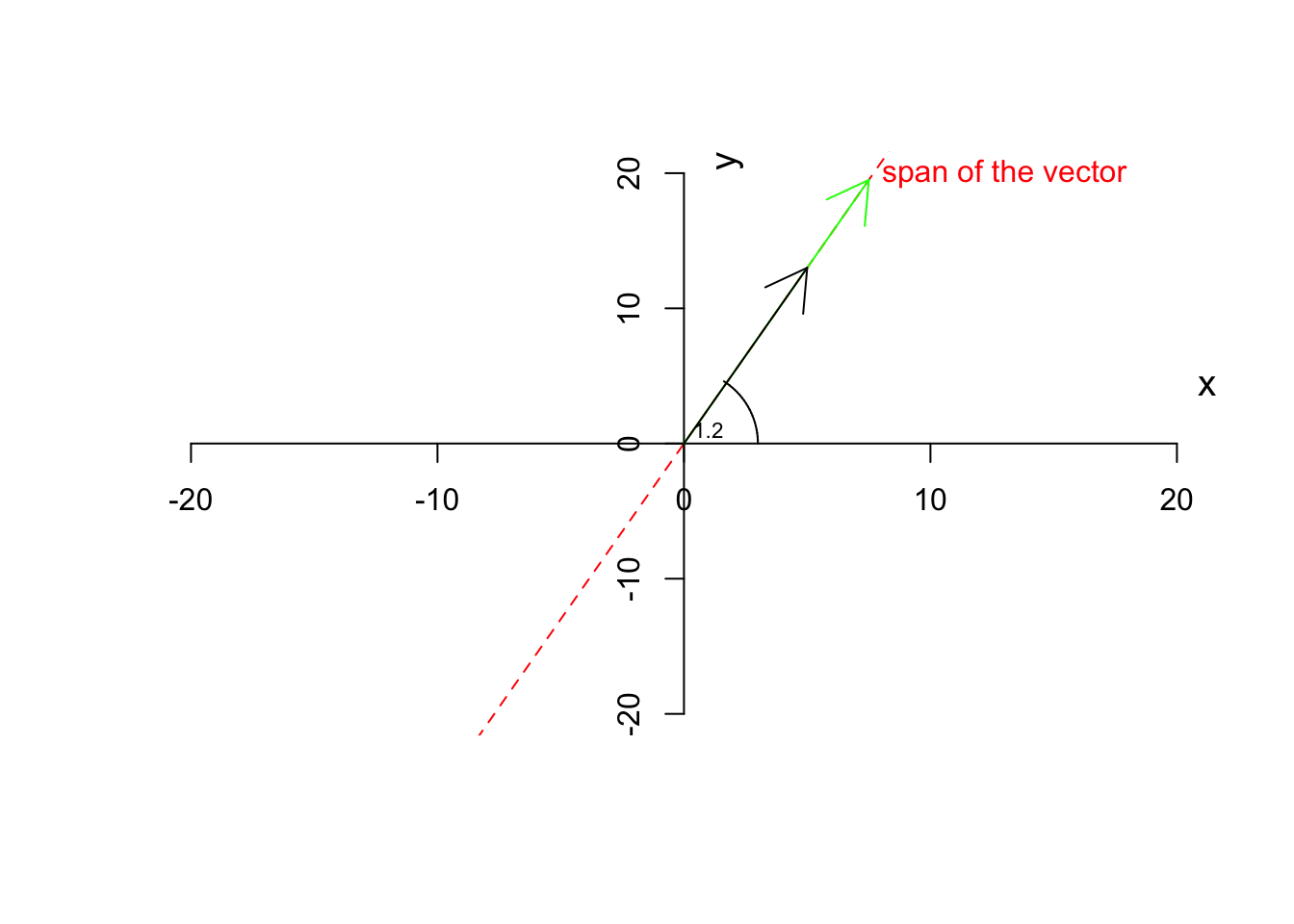
Figure 6.7: Multiplying a vector by a scalar
As you see in Figure 6.7, the green vector is the result of the multiplication of our vector by 1.5. The vector has changed magnitude (length) but not the direction. If we now multiply by \(-1.5\)
# plot the data for variable 1
plot(c(-20,20),c(-20,20),xlab = "",ylab = "",
 axes = F,type = "n")

segments(-500,-1300,500,1300,col = "red",lty = "dashed")
text(13,20,"span of the vector",col="red")


# plot the axis
axis(1,cex=4,pos = c(0,0) )
title(xlab="x", line=-10, cex.lab=1.2,adj=1)
axis(2,cex=4,pos = c(0,0) )
title(ylab="y", line=-16, cex.lab=1.2,adj=1)
# plot arrow and text

arrows(0,0,5*-1.5,13*-1.5,col="green")
arrows(0,0,5,13)

# draw circle
plotrix::draw.arc(0,0,3,angle2=1)

text(1,1,"1.2",cex=0.7)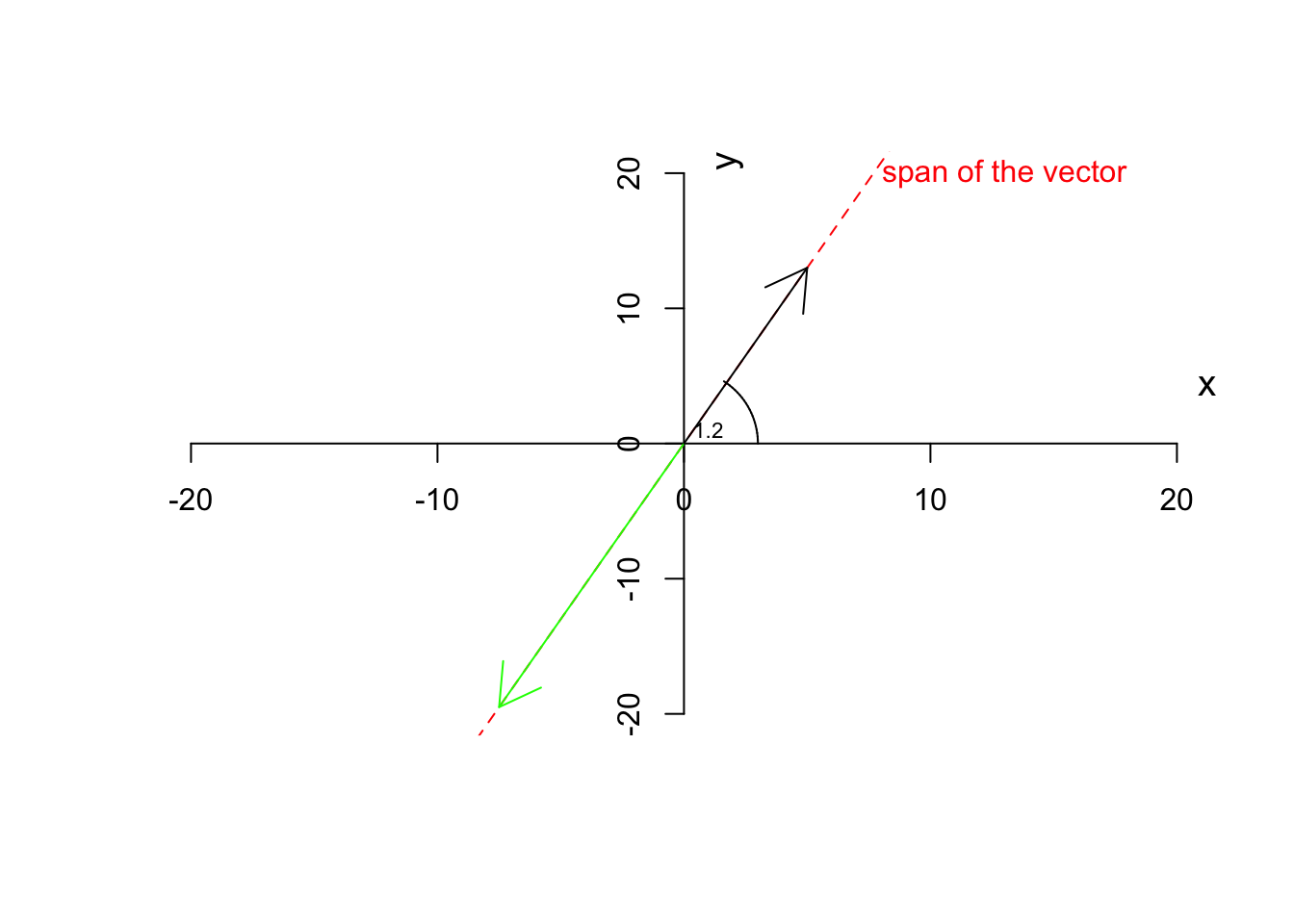
Figure 6.8: Multiplying a vector by a negative scalar
You see that the green line now points to the negative direction but still stays on the same span (the red dashed line). Let’s move on to the addition. Obviously the same applies if we add a scalar to both elements of the vector.
Now let’s have a look at when we don’t have a scalar but have a vector. Let’s start with addition and subtraction
Definition 6.6 (Vector addition and subtraction) We can add or substract two vectors only and only if they have the same number of elements. If we have \(\vec{a}=[x,y]\) and \(\vec{b}=[p,z]\) and the addition and subtraction are defined:
\[\vec{c}=\vec{a}+\vec{b}=[x+p, y+z]\]
and
\[\vec{c}=\vec{a}-\vec{b}=[x-p, y-z]\]
Obviously, we take a similar element of the vector and add or subtract them resulting to a new vector.
Let’s have a look at what it means using an example. Suppose we have two vectors, \(\vec{a}=[5,13]\) and \(\vec{b}=[3,4]\) we add them together and the result will be
\[\vec{c}=\vec{a}+\vec{b}=[5+3, 13+4]=[8,17]\] Similarly for subtraction
\[\vec{c}=\vec{a}+\vec{b}=[5-3, 13-4]=[2,9]\]
Graphically and verbally we can think about this, start with \(\vec{a}=[5,13]\), from the origin go 5 to the right and 13 up. Great! Stop here. Now let’s continue with \(\vec{b}=[3,4]\). Go 3 steps further to the right and then go 4 steps up! This is \(\vec{c}=\vec{a}+\vec{b}\)
Let’s look at the graphics:
par(mfrow=c(1,2))
# plot the data for variable 1
plot(c(-20,20),c(-20,20),xlab = "",ylab = "",
 axes = F,type = "n")

# plot the axis
axis(1,cex=4,pos = c(0,0) )
title(xlab="x", line=-10, cex.lab=1.2,adj=1)
axis(2,cex=4,pos = c(0,0) )
title(ylab="y", line=-16, cex.lab=1.2,adj=1)
# plot arrow and text

arrows(0,0,5,13,col="green")

arrows(0,0,3,4,col="red")
title("Original vectors a and b")


plot(c(-20,20),c(-20,20),xlab = "",ylab = "",
 axes = F,type = "n")


# plot the axis
axis(1,cex=4,pos = c(0,0) )
title(xlab="x", line=-10, cex.lab=1.2,adj=1)
axis(2,cex=4,pos = c(0,0) )
title(ylab="y", line=-16, cex.lab=1.2,adj=1)
# plot arrow and text
arrows(0,0,5,13,col="red")

arrows(5,13,8,17,col="green")
title("Addtion and a and b")

arrows(0,0,8,17,col="black")


# draw circle
plotrix::draw.arc(0,0,3,angle2=1)

text(1,1,"1.2",cex=0.7)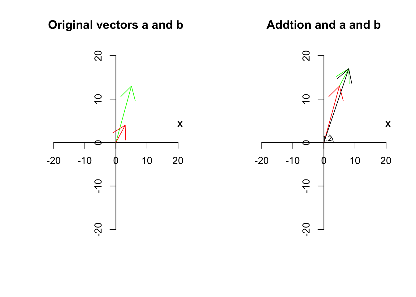
Figure 6.9: Adding two vectors
We have two vectors, \(\vec{a}\) is red, \(\vec{b}\) is green and \(\vec{c}\) is black. So the black one is the resulting vector. Has it changed span?
Let’s look at the graphics:
par(mfrow=c(1,1))
# plot the data for variable 1
plot(c(-20,20),c(-20,20),xlab = "",ylab = "",
 axes = F,type = "n")

# plot the axis
axis(1,cex=4,pos = c(0,0) )
title(xlab="x", line=-10, cex.lab=1.2,adj=1)
axis(2,cex=4,pos = c(0,0) )
title(ylab="y", line=-16, cex.lab=1.2,adj=1)
# plot arrow
arrows(0,0,8,17,col="black")

# plot span

 segments(-500,-1300,500,1300,col = "red",lty = "dashed")
text(13,20,"span of the vector a",col="red")


 segments(-300,-400,300,400,col = "green",lty = "dashed")
text(13,10,"span of the vector b",col="green")


segments(-800,-1700,800,1700,col = "black",lty = "dashed")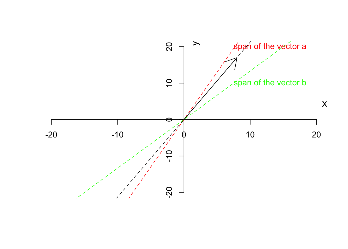
Figure 6.10: Span of vector a, b and c
You can obviously see that the span of \(\vec{c}\) (the black dashed line) is not on either of \(\vec{a}\) and \(\vec{b}\). We will later talk about why this is important. Perhaps by now, you got the point that vectors are not just a list of numbers (like an expression of a gene for 10 samples) but rather a direction and magnitude.
There are three more things to talk about before moving forward to the next section.
First thing is that we can normalize a vector to have a magnitude of 1 but keep its direction. This can be simply down by diving every element of the vector by its magnitude.
\[\frac{\vec{a}}{\|\vec{a}\|}=[\frac{x}{\|\vec{a}\|},\frac{y}{\|\vec{a}\|}]\]
This will give a normalized or unit vector which the same direction but a magnitude of 1. This is handy because we have a vector irrespective of the magnitude but we can multiply it with a scalar to go back to the same vector as we had before.
For example, if we have \(\vec{a}=[3,13]\) we can calculate its magnitude as \(\sqrt{3^2+13^2}=13.3\) giving us the unit vector of \(\hat{a}=[\frac{3}{13.3},\frac{13}{13.3}]=[0.22,0.97]\). This will come handy later when we do a PCA.
par(mfrow=c(1,1))
# plot the data for variable 1
plot(c(-10,10),c(-15,15),xlab = "",ylab = "",
 axes = F,type = "n")

# plot the axis
axis(1,cex=4,pos = c(0,0) )
title(xlab="x", line=-10, cex.lab=1.2,adj=1)
axis(2,cex=4,pos = c(0,0) )
title(ylab="y", line=-16, cex.lab=1.2,adj=1)
# plot arrow
arrows(0,0,3,13,col="black")
arrows(0,0,3/sqrt(sum(c(3,13)^2)),13/sqrt(sum(c(3,13)^2)),col="red",length = 0.1)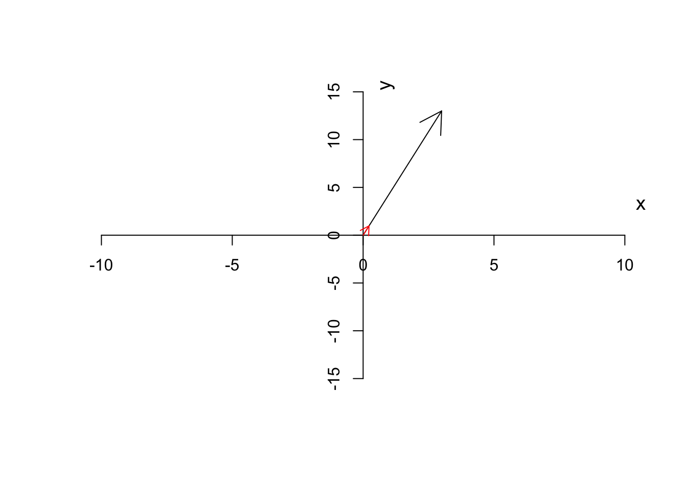
Figure 6.11: Unit vector of a has been depicted
As you see in Figure 6.11, the unit vector (red arrow) has the same direction as the original vector (black arrow) but it’s much smaller. In our example, we can multiple the unit vector to \(13.3\) to get back to the original vector as we had.
The second point is that, I guess you noted that we talked about subtraction and addition but we did not talk about the multiplication of two vectors. There are two ways to multiply two vectors. One is called cross product that is written as \(\vec{a} \times \vec{b}\) and the second one is called dot product that is written as \(\vec{a}\cdot\vec{b}\) (sometimes we don’t write the dot). Throughout this chapter, we will only talk about dot product not the cross product. But just to briefly mention it, cross-product deals with finding an orthogonal to two other lines. That is if we say \(\vec{a}=\vec{a} \times \vec{b}\), it means that \(\vec{c}\) is a line that is orthogonal to both \(\vec{a}\) and \(\vec{b}\). But Let’s ignore it and talk about the dot product.
Definition 6.7 (Dot product of two vectors) The dot product of two vectors \(\vec{a}=[x,y]\) and \(\vec{b}=[p,z]\) is define as \[d=\vec{a}\cdot\vec{b}=x \times p+y \times z\]
It might look a bit fancy, but the concept is that we would like to project or mirror vector \(\vec{a}\) onto the vector \(\vec{b}\) (or perhaps the span of \(\vec{b}\)). We take tip of the vector \(\vec{a}\), draw an orthogonal line from the time to the vector \(\vec{b}\), this gives us the location of vector \(\vec{a}\) on \(\vec{b}\), let’s call this new location \(\vec{d}\), we now extend the vector \(\vec{d}\) by the magnitude of \(\|\vec{b}\|\).
Ok! That was a little bit too much. Let’s look at an example to make this clear.
Let’s draw vector \(\vec{a}\) and \(\vec{b}\)
par(mfrow=c(1,1))
# plot
plot(c(-5,40),c(-2,10),xlab = "",ylab = "",
 axes = F,type = "n")


# plot arrow b
arrows(0,0,20,0,col="blue")
# write b
text(10,-2,labels = "b",col="blue")


# plot arrow b
arrows(0,y0 = 0,8,10,col="red")
# write a
text(4,10,labels = "a",col="red")

segments(8,10,8,0,lty = "dashed")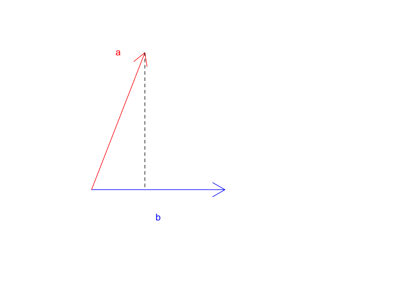
Figure 6.12: Two vectors a and b
Great! Where does \(\vec{a}\) land if it starts falling down? Now let’s take the tip of the \(\vec{a}\) and draw a line perpendicular to \(\vec{b}\).
par(mfrow=c(1,1))
# plot
plot(c(-5,40),c(-2,10),xlab = "",ylab = "",
 axes = F,type = "n")


# plot arrow b
arrows(0,0,20,0,col="blue")
# write b
text(18,-1,labels = "b",col="blue")


# plot arrow b
arrows(0,y0 = 0,8,10,col="red")
# write a
text(4,10,labels = "a",col="red")
# draw lines and arrows
segments(8,10,8,0,lty = "dashed")
text(20,6,labels = "perpendicular line (projection line)",col="black")
arrows(4,-1,8, 0,col="black")
text(2,-1.5,labels = "projection location",col="black")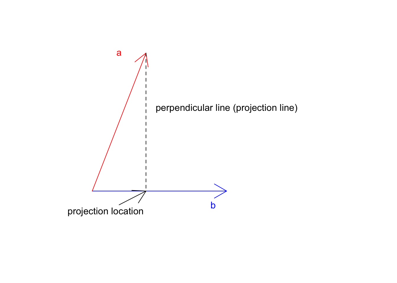
Figure 6.13: Two vectors a and b
Now we know the location \(\vec{a}\) on \(\vec{b}\) this is exactly at 8 we can go ahead and multiply this but the magnitude of \(\vec{b}\) (20):
par(mfrow=c(1,1))
# plot
plot(c(-5,165),c(-2,10),xlab = "",ylab = "",
 axes = F,type = "n")


# plot arrow b
arrows(0,0,20,0,col="blue")
# write b
text(18,-1,labels = "b",col="blue")


# plot arrow b
arrows(0,y0 = 0,8,10,col="red")
# write a
text(4,10,labels = "a",col="red")
# draw lines and arrows
segments(8,10,8,0,lty = "dashed")

text(50,6,labels = "perpendicular line (projection line)",col="black")

arrows(4,-1,8, 0,col="black")

text(10,-1.5,labels = "projection location",col="black")


arrows(0,0,8*sqrt(sum(c(20,0)^2)),0,col="red",lty = "dashed")

text(150,-2,labels = "dot product of a.b",col="red")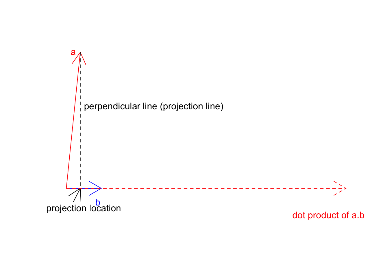
Figure 6.14: Two vectors a and b
So the dot product of \(\vec{a}\) on \(\vec{b}\) will be that dashed red line. One way to think about the whole concept as we have two different cells with different growth rates. We take cell a with some growth apply b growth to it. So if a is already going 2x, and b is going 3 we take 2 and make it 3 times larger! You will see soon that when we work with unit vectors (magnitude of 1), everything becomes much clearer.
The last thing we want to discuss about the vector is the definition of space (6.2). At that point, we did not know much about the vectors. We now can re-define our space as a vector space. The vector space is the set of all possible vectors that we can draw for our dimensions. So far we have been working on two dimensions and we said that we can think about each dimension as a gene or any kind of measurement of interest. Let’s consider two genes that can be either silent (zero) or have positive expressions. In reality, we barely know the extend of expression of one gene. It might go from zero to some unknown number. But let’s assume that it can go all the way to 20. Now we are given all the power in the world to be able to induce gene expression to create a human (based on two genes only). Since we know some good deal of linear algebra by now, it’s not that difficult! I can go ahead and say I have a person and gene 1=15 and gene 2=5.
par(mfrow=c(1,1))
# plot
plot(c(0,20),c(0,20),xlab = "Gene 1",ylab = "Gene 2",
 axes = T,type = "n")
# plot arrow b
arrows(0,0,15,5,col="blue")
# add point
points(15,5)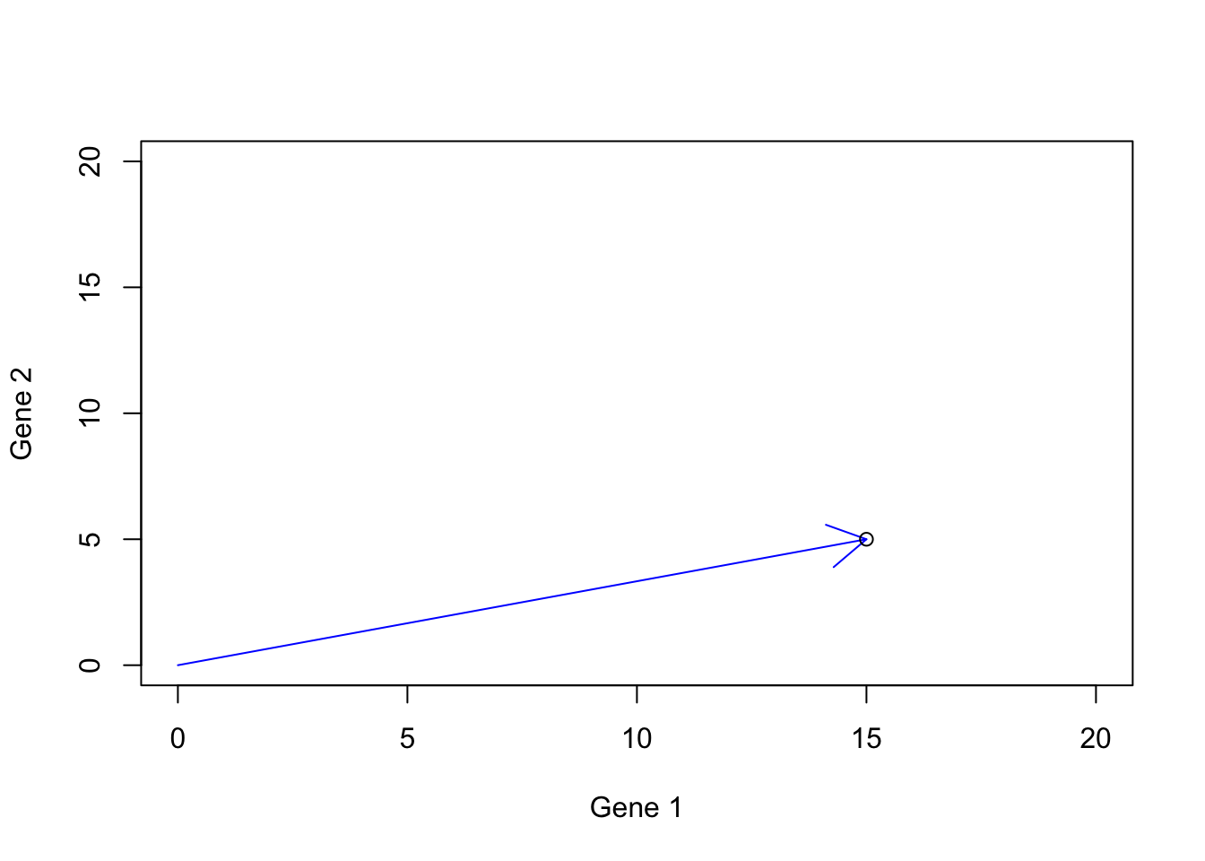
Figure 6.15: Gene expression example
If we think a bit, we see that we can create so many humans by these two genes.
par(mfrow=c(1,1))
# plot
plot(c(0,20),c(0,20),xlab = "Gene 1",ylab = "Gene 2",
 axes = T,type = "n")

#Draw arrows
for(i in 1:100)
{
  set.seed(i)
  g1<-sample(1:20,1)
   set.seed(i*100)
  g2<-sample(1:20,1)
  # plot arrow b
arrows(0,0,g1,g2,col="blue")
# add point
points(g1,g2)
}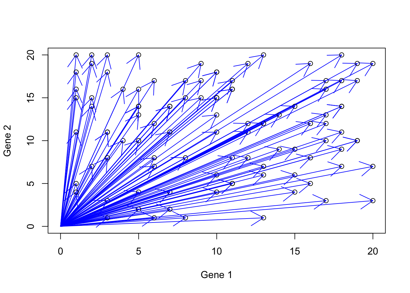
Figure 6.16: Gene expression example with more vectors
These possible values are in fact part of your vector spaces. Essentially all the vectors that can be created are located in this space. The power we were given to work with such space and create what we want was already covered. Our tools are vector addition, subtraction, scalar multiplication, and possible dot product. There is only one thing left. We need two buffers, each container the two genes that we can activate/deactivate (ONE at the time), induce the expression, mix the buffers, and create a human! Our First buffer we call b1 is contains both gene 1 and 2, but gene 2 is deactivated, giving us \(b1=[gene1,gene2]\). Let’s say we want to represent activated gene by 1 and deactivated gene by zero so b1 one becomes \(b1=[1,0]\). Let’s do the same thing for our second buffer, \(b2=[gene1,gene2]\) and turn gene1 to off, \(b1=[0,1]\). Let’s again say that we want to create a human (\(h\)) with gene1=15 and gene2=5 so our sample should \(h=[15,5]\). With the tools that we are given and two buffers \(b1=[1,0]\) and \(b2=[0,1]\) how can we reach to \(h=[15,5]\)?
Well, that is not that difficult.
Let’s induce gene 1 and call it \(b1i\): \(b1i=15 \times b1=[15 \times 1, 15 \times 0]=[15,0]\). Perfect. We induced the first gene but scalar multiplication. Now we do this for the second gene and call it \(b2i\): \(b2i=5 \times b2=[5 \times 0, 5 \times 1]=[0,5]\). We now have gene 2 again with scalar multiplication. How can we mix these two genes and make our first human: \(h=b1i+b2i=[15+0,5+0]=[15,5]\). Yess! We made it!
These small raw vectors (\(\vec{b1}\) and \(vec{b2}\)) together with our operations (addition, multiplication, etc) help us to create any possible vector in our space. These are basis vectors.
Definition 6.8 (Basis vectors) The basis vectors are a set of vectors that when used in weighted combination can create any vector in our space. In fact our space itself is defined by the basis vectors. To be called the basis vector, these should be pointing to different directions. To be more concrete, the basis vectors should be linearly independent, meaning that they cannot be created by a combination of other vectors.
Our “default” basis vectors are x=[1,0] and y=[0,1]. That is the only reason that when we plot any data in for example R, the values of our measurements will be plotted exactly as they are. If we assume anything else than x=[1,0] and y=[0,1], our plot will end up being something else. So in short, the default basis vector, let us moving around our space to any point and also show us the original angle of our data. We will see later that we can change these basis vectors in order to rotate our data and see another angle of them. So far let’s agree that our basis is [0,1] and [1,0] and they are used to construct our data vectors. We can think about this, with the help of our data change direction, and magnitude of the basis vectors in order to represent our data in the space defined by the basis vectors.
Let’s have a look at the previous example. We start with two basis vectors \(\vec{b1}=[1,0]\) (blue arrow) and \(\vec{b2}=[0,1]\) (green arrow). Our aim was to reach the vector \(\vec{h}=[15,5]\) (black point):
par(mfrow=c(1,1))
# plot
plot(c(-1,15),c(-1,10),xlab = "Gene 1",ylab = "Gene 2",
 axes = T,type = "n")

# draw arrows and text
arrows(0,0,1,0,col="blue",length = 0.1)
text(0.5,-0.5,"b1",col="blue")

arrows(0,0,0,1,col="red",length = 0.1)
text(-0.5,0.5,"b2",col="red")

# Draw plot
points(15,5)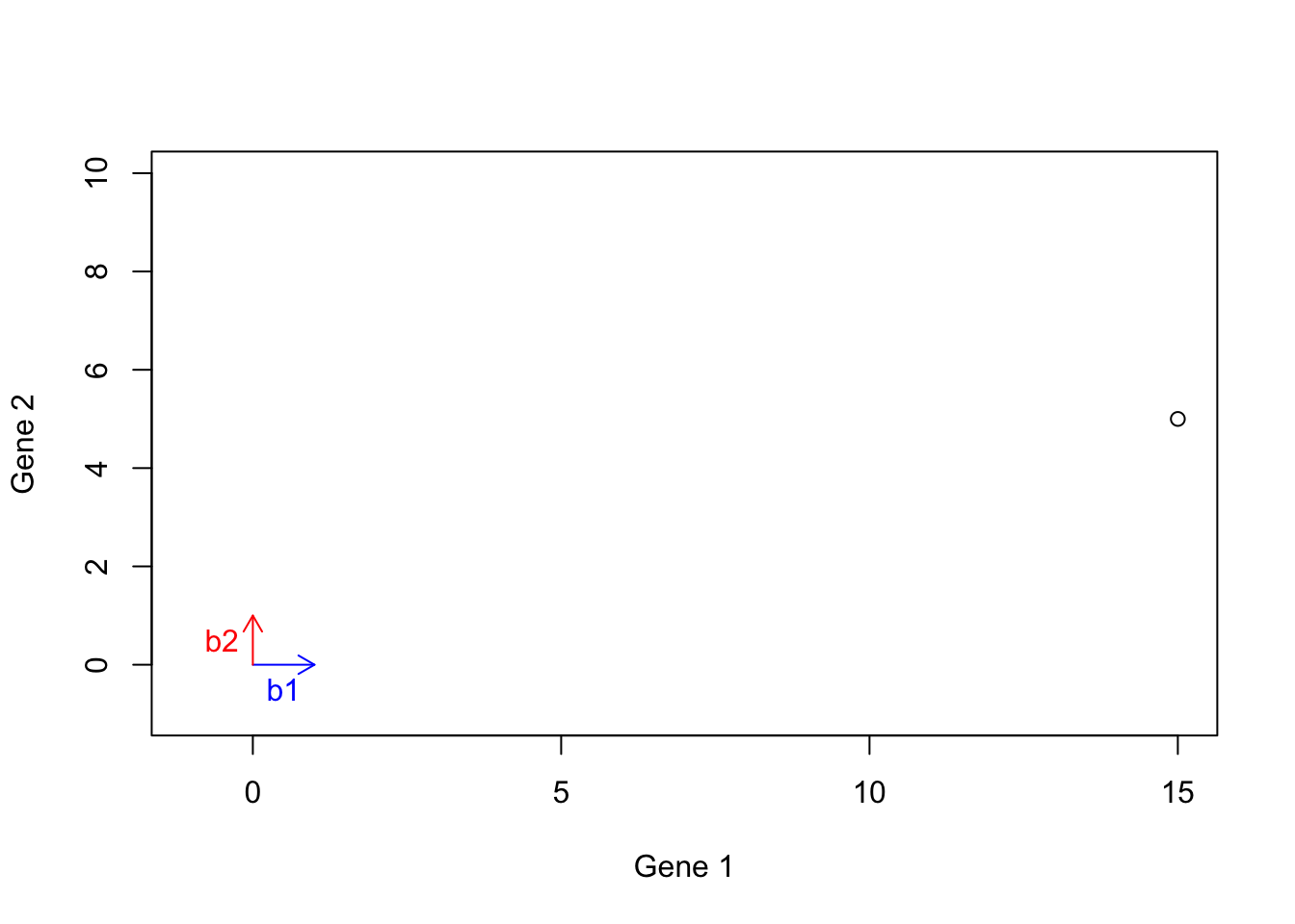
Figure 6.17: Example of basis vectors
We first calculate this: \(b1i\): \(b1i=15 \times b1=[15 \times 1, 15 \times 0]=[15,0]\), giving us the dashed arrow:
par(mfrow=c(1,1))
# plot
plot(c(-1,15),c(-1,10),xlab = "Gene 1",ylab = "Gene 2",
 axes = T,type = "n")
# draw arrows
arrows(0,0,15,0,col="blue",length = 0.1,lty = "dashed")
text(7,-0.5,"b1i",col="blue")

arrows(0,0,0,1,col="red",length = 0.1)
text(-0.5,0.5,"y",col="red")
# put point
points(15,5)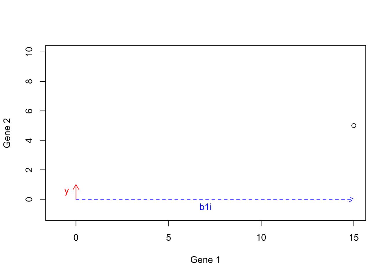
Figure 6.18: Example of basis vectors (scale b1)
We then calculate \(b2i\): \(b2i=5 \times b2=[5 \times 0, 5 \times 1]=[0,5]\):
par(mfrow=c(1,1))
# plot
plot(c(-1,15),c(-1,10),xlab = "Gene 1",ylab = "Gene 2",
 axes = T,type = "n")
# draw arrows
arrows(0,0,15,0,col="blue",length = 0.1,lty = "dashed")
text(7,-0.5,"b1i",col="blue")

arrows(0,0,0,5,col="red",length = 0.1,lty = "dashed")
text(-0.5,2.5,"b2i",col="red")

points(15,5)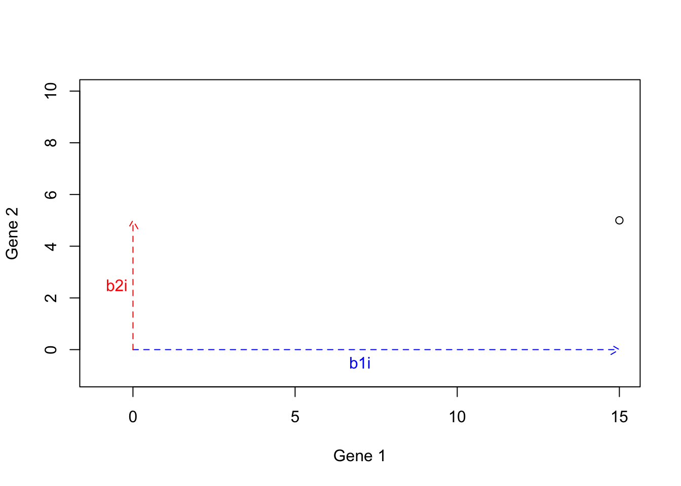
Figure 6.19: Example of basis vectors (scale b2)
We can now calculate \(h=b1i+b2i=[15+0,5+0]=[15,5]\):
par(mfrow=c(1,1))
# plot
plot(c(-1,15),c(-1,10),xlab = "Gene 1",ylab = "Gene 2",
 axes = T,type = "n")
# draw arrows
arrows(0,0,15,0,col="blue",length = 0.1,lty = "dashed")
text(7,-0.5,"b1i",col="blue")

arrows(15,0,15,5,col="red",length = 0.1,lty = "dashed")
text(14.5,2.5,"b2i",col="red")

points(15,5)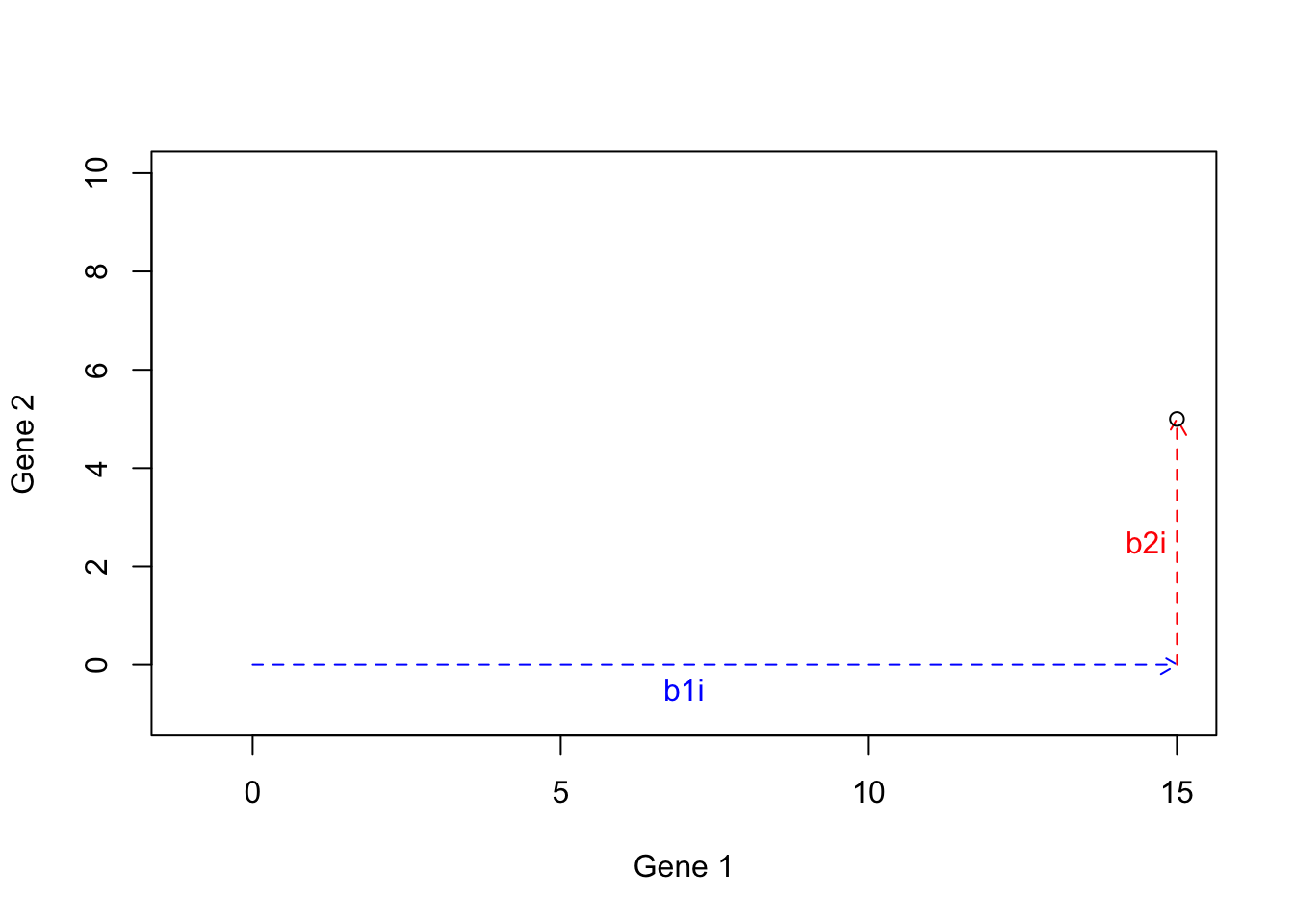
Figure 6.20: Example of basis vectors (b1i+b2i)
We can now draw a line from the origin to the tip of \(b1i+b2i\):
par(mfrow=c(1,1))
# plot
plot(c(-1,15),c(-1,10),xlab = "Gene 1",ylab = "Gene 2",
 axes = T,type = "n")
# draw arrows
arrows(0,0,15,0,col="blue",length = 0.1,lty = "dashed")
text(7,-0.5,"b1i",col="blue")

arrows(15,0,15,5,col="red",length = 0.1,lty = "dashed")
text(14.5,2.5,"b2i",col="red")

arrows(0,0,15,5,col="black",length = 0.1,lty = "dashed")
text(8,3.5,"h",col="black")

points(15,5)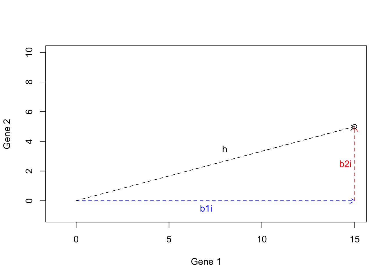
Figure 6.21: Example of basis vectors (calculating h)
I hope that you got the point by now. We can use the basis vectors to construct any vector in our space. In fact, our observations vectors (e.g. samples) are basis vectors that have been scaled and added.
We come to the end of the vector section. The important point here is that we have been working on two dimensions, all the operations and concepts discussed so far can be extended to work in a high dimension. Remember our dataset had 45101 dimensions. We have only worked on two of them so far :)
6.4 Matrices
Matrices can be thought of as a generalization of vectors where we put multiple vectors together to form a “table”. You can think about an Excel sheet where each row or each column is a vector but the complete sheet is a matrix. We normally store our data in matrices as we showed in Table 4.1. As you noticed, matrices have can have columns and rows. These are dimensions of a matrix. In our test data, we dimension is
## [1] 23 45101Throughout this section, we show matrices with capital letters as opposed to vectors that are shown using small letters. \[ A=\begin{bmatrix} 1 & 2 & 3\\ 4 & 5 & 6 \end{bmatrix} \] As you see, we have two rows and three columns. When we want to refer to a specific location (called entry) in the matrix, we use i for the row index and j for the column index.
For example \(A_{1,2}\) refers to an entry sitting in the first frow and the **second column of the matrix, giving us \(2\).
We refer to the entire row of the matrix by i,*. For example, \(A_{2,*}\) will give us \([4,5,6]\). In the same way, we can refer to the entire column \(A_{*,2}\), giving us \([2,5]\).
Many of the operations defined for the vectors are also applied on the matrices. We can add or subtract them but the important thing is that the matrices MUST be the same size (same dimensions) to be able to perform addition and subtraction. In the case of addition and subtraction, each entry of the first matrix will be added or substracted to the same entry (same location) in the second matrix:
\[ \begin{bmatrix} 1 & 2 & 3\\ 4 & 5 & 6 \end{bmatrix}+ \begin{bmatrix} 7 & 8 & 9\\ 10 & 11 & 12 \end{bmatrix}= \begin{bmatrix} 1+7 & 2+8 & 3+9\\ 4+10 & 5+11 & 6+12 \end{bmatrix} \] The same applies in scalar multiplication:
\[ 5 \times \begin{bmatrix} 1 & 2 & 3\\ 4 & 5 & 6 \end{bmatrix}= \begin{bmatrix} 5 \times 1 & 5 \times 2 & 5 \times 3\\ 5 \times 4 & 5 \times 5 & 5 \times 6 \end{bmatrix} \] We can think about addition, subtraction, and scalar multiplication the same way as the vectors. However, instead of having one vector, we have multiple ones.
For example, if we add \(A=\begin{bmatrix}2&4\\5&3\end{bmatrix}\) and \(B=\begin{bmatrix}4&5\\2&2\end{bmatrix}\) we will get \(C=\begin{bmatrix}6&9\\7&5\end{bmatrix}\). We can think about we have two genes (number of columns) and we have two patients (number of rows) in \(A\) and \(B\). Each patient will give us an arrow.
#
par(mfrow=c(2,2))
# define matrices
A<-matrix(c(2,4,5,3),nrow = 2,ncol = 2,byrow = T)

B<-matrix(c(4,5,2,2),nrow = 2,ncol = 2,byrow = T)

C=A+B

# Plot arrows in A
plot(c(0,10),c(0,10),xlab = "",ylab = "",
 axes = T,type = "n")
title("Matrix A")
# draw arrows
arrows(0,0,A[1,1],A[1,2],col="blue",length = 0.1)
text(A[1,1]/2,A[1,2]/2,expression('A'["1,*"]),col="blue",adj = -0.5)

arrows(0,0,A[2,1],A[2,2],col="red",length = 0.1)
text(A[2,1]/2,A[2,2]/2,expression('A'["2,*"]),col="red",adj = -0.5)

# Plot arrows in B
plot(c(0,10),c(0,10),xlab = "",ylab = "",
 axes = T,type = "n")
title("Matrix B")

arrows(0,0,B[1,1],B[1,2],col="green",length = 0.1)
text(B[1,1]/2,B[1,2]/2,expression('B'["1,*"]),col="green",adj = -0.5)

arrows(0,0,B[2,1],B[2,2],col="purple",length = 0.1)
text(B[2,1]/2,B[2,2]/2,expression('B'["2,*"]),col="purple",adj = -0.5)

# Plot arrows in A+b
plot(c(0,10),c(0,10),xlab = "",ylab = "",
 axes = T,type = "n")
title("Matrix A+B")

# draw arrows
arrows(0,0,A[1,1],A[1,2],col="blue",length = 0.1)
text(A[1,1]/2,A[1,2]/2,expression('A'["1,*"]),col="blue",adj = -0.5)

arrows(0,0,A[2,1],A[2,2],col="red",length = 0.1)
text(A[2,1]/2,A[2,2]/2,expression('A'["2,*"]),col="red",adj = -0.5)


arrows(A[1,1],A[1,2],C[1,1],C[1,2],col="green",length = 0.1,lty = "dashed")
text(C[1,1]/2,C[1,2]/2,(expression('B'["1,*"])),col="green")

arrows(A[2,1],A[2,2],C[2,1],C[2,2],col="purple",length = 0.1,lty = "dashed")
text(C[2,1]/2,C[2,2]/2,(expression('B'["2,*"])),col="purple",adj = -2)


## plot C
plot(c(0,10),c(0,10),xlab = "",ylab = "",
 axes = T,type = "n")
title("Matrix C")
arrows(0,0,C[1,1],C[1,2],col="blue",length = 0.1)
text(C[1,1]/2,C[1,2]/2,expression('C'["1,*"]),col="blue",adj = -0.5)

arrows(0,0,C[2,1],C[2,2],col="red",length = 0.1)
text(C[2,1]/2,C[2,2]/2,expression('C'["2,*"]),col="red",adj = -0.5)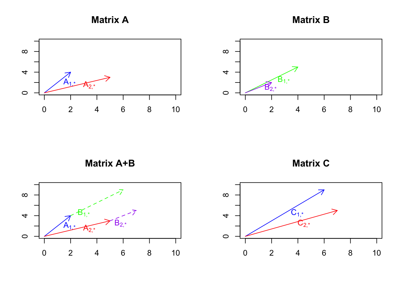
Figure 6.22: Example of matrix addition
So what we see in Figure 6.22 is that we have two matrices A and B, we take the vectors in B and put them at the tip of the vectors in A, we then draw two lines from the origin to the new tips of B. So as it’s obvious now, this is the same and vector addition we just do it for more vectors.
6.4.1 Matrix multiplication
In order to understand matrix multiplication, we have to think about the space again. If you remember, we said the we can represent our space by the basis vector \(\vec{x}=[1,0]\) and \(\vec{y}=[0,1]\). We can think about this as directions or our guide to move to any points in the space. We said that we can scale them, we can add/subtract them to represent any vectors in the space. Our space is an empty huge place wherein we just put our vectors! The way that we navigate in space, is just by scaling and adding and subtracting the basis vectors. I keep repeating this because it’s important to understand it thoroughly. So let’s have a look at our empty space (well, I just put the grid so we have a feeling of it)
par(mfrow=c(1,1))
# define data
mydata<-cbind(-5:5,rep(-5,11),-5:5,rep(5,11))

mydata2<-cbind(rep(-5,11),-5:5,rep(5,11),-5:5)
# Plot
plot(range(rbind(mydata[,1],mydata[,3])),range(rbind(mydata[,2],mydata[,4])),
     type="n",xlab="",ylab="",xlim=c(-5,5),ylim=c(-5,5),axes = F,bg="black")


# Draw lines
nl<-apply(mydata,MARGIN = 1,function(x){
  segments(x[1],x[2],x[3],x[4])})

nl<-apply(mydata2,MARGIN = 1,function(x){
  segments(x[1],x[2],x[3],x[4])})

# Draw arrows
arrows(0,0,1,0,col="red",length=0.1)
arrows(0,0,0,1,col="blue",length=0.1)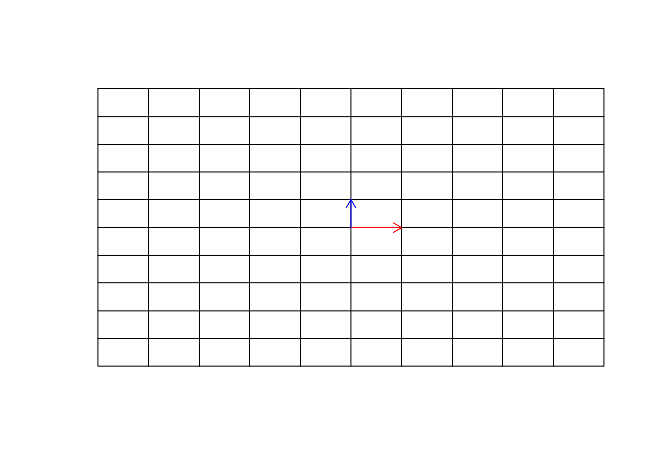
Figure 6.23: Empty space
We can go to any point on this grid, simply using our basis vectors.
par(mfrow=c(1,1))

# Define data
mydata<-cbind(-5:5,rep(-5,11),-5:5,rep(5,11))

mydata2<-cbind(rep(-5,11),-5:5,rep(5,11),-5:5)

plot(range(rbind(mydata[,1],mydata[,3])),range(rbind(mydata[,2],mydata[,4])),
     type="n",xlab="",ylab="",xlim=c(-5,5),ylim=c(-5,5),axes = F,bg="black")

# Draw lines
nl<-apply(mydata,MARGIN = 1,function(x){
  segments(x[1],x[2],x[3],x[4])})

nl<-apply(mydata2,MARGIN = 1,function(x){
  segments(x[1],x[2],x[3],x[4])})

# Draw arrows
arrows(0,0,1,0,col="red",length=0.1)
arrows(0,0,0,1,col="blue",length=0.1)

points(4,3,col="purple",pch=7)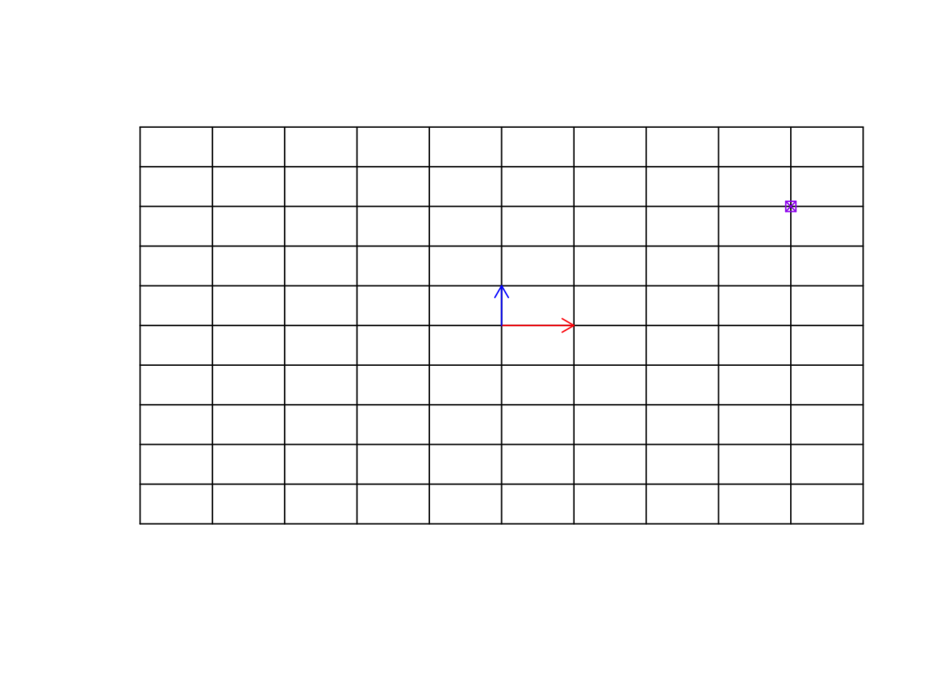
Figure 6.24: Empty space and a target point
Remember now, this target point can be an observation (e.g. sample, etc). We can move to this point simply by multiplying \(\vec{x}\) to 4 and \(\vec{y}\) to 3 and then add the resulting vectors, giving us the location of the purple point \([4,3]\).
par(mfrow=c(1,1))
# Define data
mydata<-cbind(-5:5,rep(-5,11),-5:5,rep(5,11))

mydata2<-cbind(rep(-5,11),-5:5,rep(5,11),-5:5)
# plot data
plot(range(rbind(mydata[,1],mydata[,3])),range(rbind(mydata[,2],mydata[,4])),
     type="n",xlab="",ylab="",xlim=c(-8,8),ylim=c(-8,8),axes = F,bg="black")

# Draw lines
nl<-apply(mydata,MARGIN = 1,function(x){
  segments(x[1],x[2],x[3],x[4])})

nl<-apply(mydata2,MARGIN = 1,function(x){
  segments(x[1],x[2],x[3],x[4])})

# Draw arrows
arrows(0,0,1,0,col="red",length=0.1,)
arrows(0,0,0,1,col="blue",length=0.1)

points(4,3,col="purple",pch=7)
arrows(0,0,4,3,col="purple",length=0.1)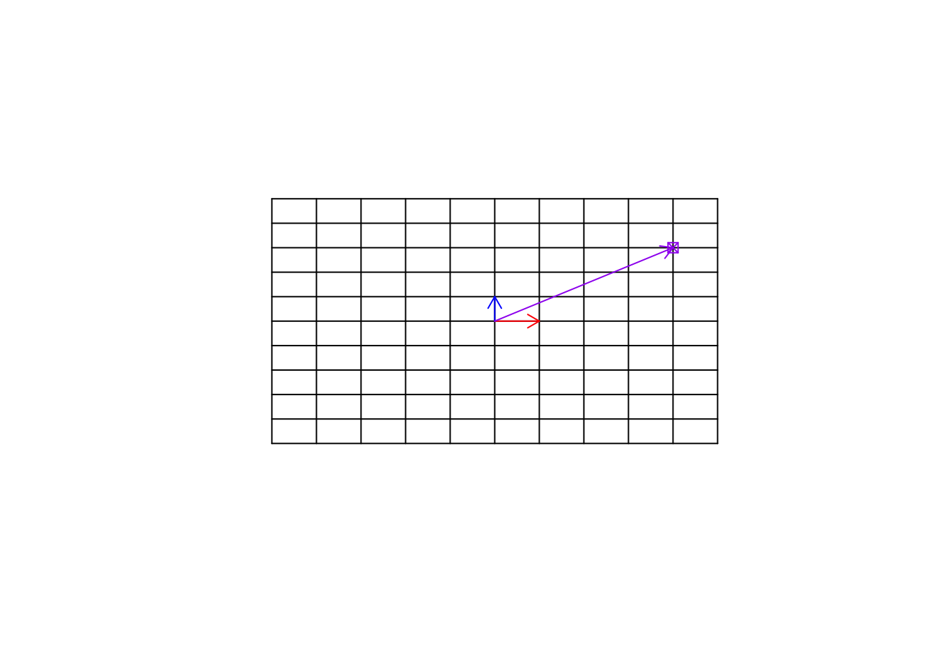
Figure 6.25: Empty space and a target point
So far we have only changed the vectors. But we can also change the space itself. If we multiply a matrix to space itself, we change the space. You can think about this like stretching, squeezing, etc applied on the whole grid and ALL the things on that grid. It might not be very understandable in the beginning. Let’s have a look at an example.
par(mfrow=c(1,1))
# Define data
mydata<-cbind(-5:5,rep(-5,11),-5:5,rep(5,11))

mydata2<-cbind(rep(-5,11),-5:5,rep(5,11),-5:5)

# Plot
plot(range(rbind(mydata[,1],mydata[,3])),range(rbind(mydata[,2],mydata[,4])),
     type="n",xlab="",ylab="",xlim=c(-8,8),ylim=c(-8,8),axes = F,bg="black")


b<-as.matrix(data.frame(a=c(1,0),b=c(1,2)))
# calculate the transformation
mydata[,c(1,2)]<-t(b%*%t(mydata[,c(1,2)]))
mydata[,c(3,4)]<-t(b%*%t(mydata[,c(3,4)]))

mydata2[,c(1,2)]<-t(b%*%t(mydata2[,c(1,2)]))
mydata2[,c(3,4)]<-t(b%*%t(mydata2[,c(3,4)]))

# Draw lines
nl<-apply(mydata,MARGIN = 1,function(x){
  segments(x[1],x[2],x[3],x[4])})

nl<-apply(mydata2,MARGIN = 1,function(x){
  segments(x[1],x[2],x[3],x[4])})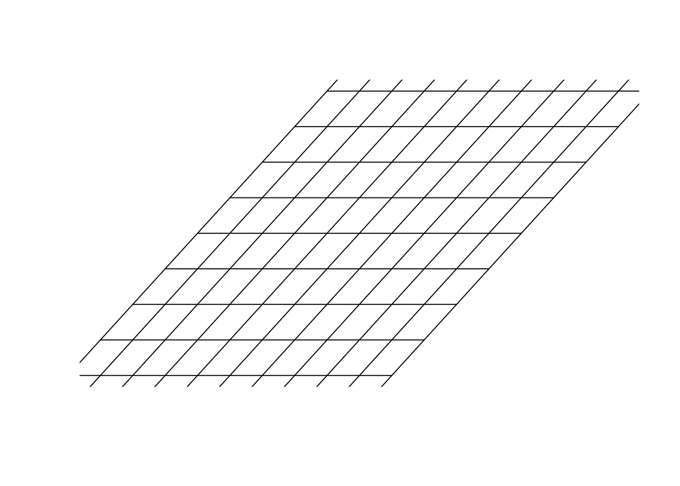
Figure 6.26: Multiply a matrix to space
In figure 6.26, we multiply \(\begin{bmatrix}1&1\\0&2\end{bmatrix}\) to our space. Please remember, we agreed before that our space was defined by \(\vec{x}=[1,0]\) and \(\vec{y}=[0,1]\) and for clarification, we plotted all the parallel lines (grid) to \(\vec{x}=[1,0]\) and \(\vec{y}=[0,1]\). Isn’t this awesome?! We can transform the space itself. We are in a transformed world! How do we find the new address (location) of the previous point (the purple one) in this new world? Well, the only thing we need, is our guides. The new location of the basis vectors. Once we get them, we can use them to find the new address. Let’s find them:
par(mfrow=c(1,1))

# Data
mydata<-cbind(-5:5,rep(-5,11),-5:5,rep(5,11))

mydata2<-cbind(rep(-5,11),-5:5,rep(5,11),-5:5)

# Plot
plot(range(rbind(mydata[,1],mydata[,3])),range(rbind(mydata[,2],mydata[,4])),
     type="n",xlab="",ylab="",xlim=c(-8,8),ylim=c(-8,8),axes = F,bg="black")


b<-as.matrix(data.frame(a=c(1,0),b=c(1,2)))
# calculate the transformation
mydata[,c(1,2)]<-t(b%*%t(mydata[,c(1,2)]))
mydata[,c(3,4)]<-t(b%*%t(mydata[,c(3,4)]))

mydata2[,c(1,2)]<-t(b%*%t(mydata2[,c(1,2)]))
mydata2[,c(3,4)]<-t(b%*%t(mydata2[,c(3,4)]))

# draw lines
nl<-apply(mydata,MARGIN = 1,function(x){
  segments(x[1],x[2],x[3],x[4])})

nl<-apply(mydata2,MARGIN = 1,function(x){
  segments(x[1],x[2],x[3],x[4])})

arrows(0,0,1,0,col="red",length=0.1,)
arrows(0,0,1,2,col="blue",length=0.1)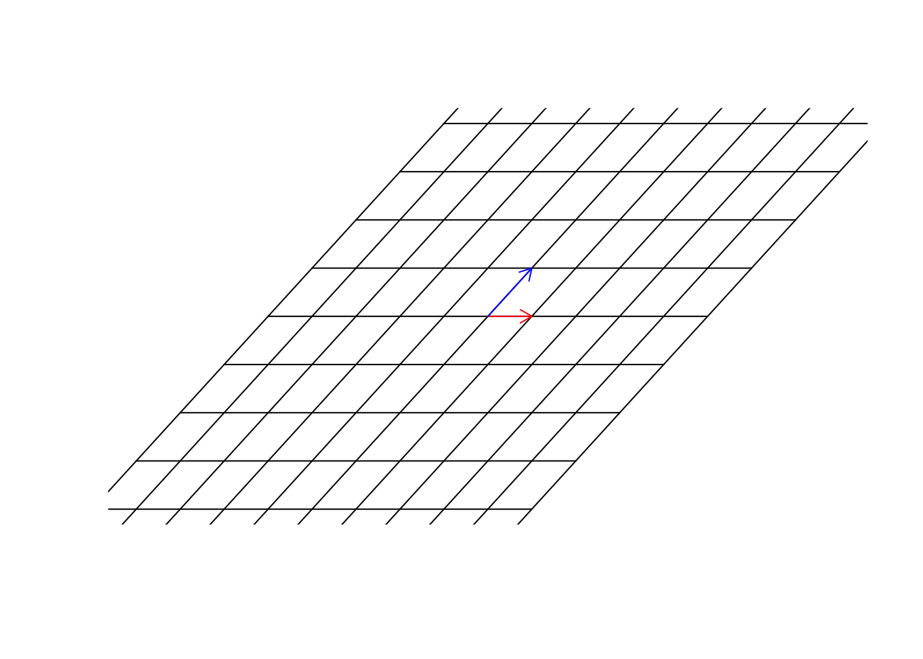
Figure 6.27: Multiply a matrix to space, including the basis vectors
Now we have them. Great. In this new world, \(\vec{x}=[1,0]\) so unchanged but \(\vec{y}=[1,2]\). Now we use the same address as before. We said that we multiple \(\vec{x}\) to 4, so it becomes, \(\vec{x}=[4,0]\) and we multiply \(\vec{y}\) to 3 so it becomes \(\vec{y}=[3,6]\). Now we add them \(\vec{x}+\vec{y}=[7,6]\). This is the address of the same point in the new world!
par(mfrow=c(1,1))
# data
mydata<-cbind(-5:5,rep(-5,11),-5:5,rep(5,11))

mydata2<-cbind(rep(-5,11),-5:5,rep(5,11),-5:5)
# plot
plot(range(rbind(mydata[,1],mydata[,3])),range(rbind(mydata[,2],mydata[,4])),
     type="n",xlab="",ylab="",xlim=c(-8,8),ylim=c(-8,8),axes = F,bg="black")


b<-as.matrix(data.frame(a=c(1,0),b=c(1,2)))
# calculate the transformation
mydata[,c(1,2)]<-t(b%*%t(mydata[,c(1,2)]))
mydata[,c(3,4)]<-t(b%*%t(mydata[,c(3,4)]))

mydata2[,c(1,2)]<-t(b%*%t(mydata2[,c(1,2)]))
mydata2[,c(3,4)]<-t(b%*%t(mydata2[,c(3,4)]))
# lines
nl<-apply(mydata,MARGIN = 1,function(x){
  segments(x[1],x[2],x[3],x[4])})

nl<-apply(mydata2,MARGIN = 1,function(x){
  segments(x[1],x[2],x[3],x[4])})

arrows(0,0,(b%*%c(1,0))[1],(b%*%c(1,0))[2],col="red",length=0.1,)
arrows(0,0,(b%*%c(0,1))[1],(b%*%c(0,1))[2],col="blue",length=0.1)

points((b%*%c(4,3))[1],(b%*%c(4,3))[2],col="purple",pch=7)
arrows(0,0,(b%*%c(4,3))[1],(b%*%c(4,3))[2],col="purple",length=0.1)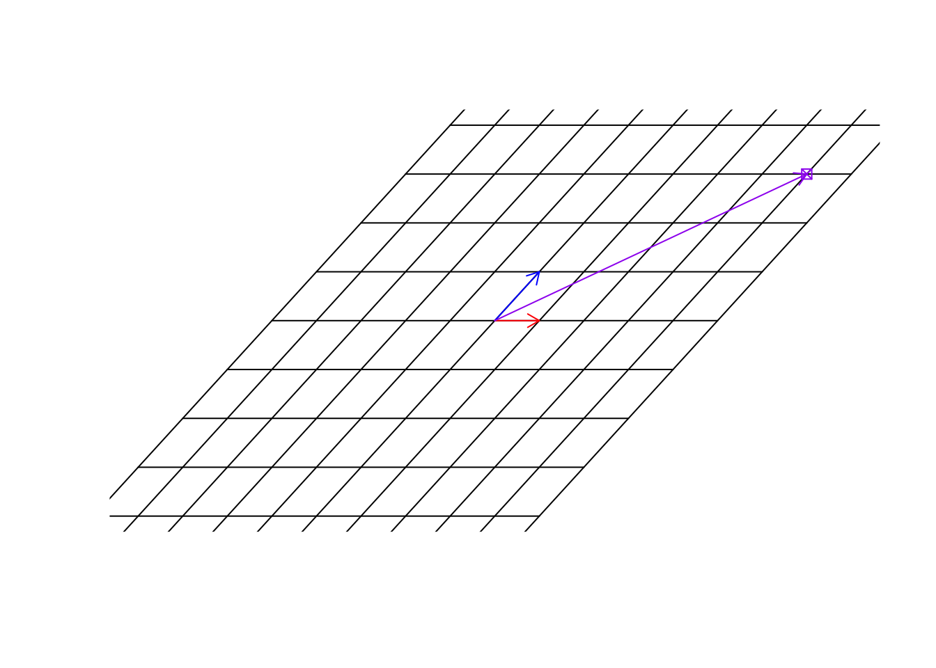
Figure 6.28: Location of the target point
So to put it simply, we just changed our coordinate system. The way we use to move around space has changed. The only way to find the location of the previous point is to know what transformation has been done to space and what happened to our basis.
Let’s have a look at another transformation.
par(mfrow=c(1,1))
# data
mydata<-cbind(-5:5,rep(-5,11),-5:5,rep(5,11))

mydata2<-cbind(rep(-5,11),-5:5,rep(5,11),-5:5)
# plot
plot(range(rbind(mydata[,1],mydata[,3])),range(rbind(mydata[,2],mydata[,4])),
     type="n",xlab="",ylab="",xlim=c(-8,8),ylim=c(-8,8),axes = F,bg="black")


tet<-2
b<-matrix(c(cos(tet),sin(tet),-sin(tet),cos(tet)),nrow = 2,byrow = T)
# calculate the transformation
mydata[,c(1,2)]<-t(b%*%t(mydata[,c(1,2)]))
mydata[,c(3,4)]<-t(b%*%t(mydata[,c(3,4)]))

mydata2[,c(1,2)]<-t(b%*%t(mydata2[,c(1,2)]))
mydata2[,c(3,4)]<-t(b%*%t(mydata2[,c(3,4)]))
# lines and arrows
nl<-apply(mydata,MARGIN = 1,function(x){
  segments(x[1],x[2],x[3],x[4])})

nl<-apply(mydata2,MARGIN = 1,function(x){
  segments(x[1],x[2],x[3],x[4])})

arrows(0,0,(b%*%c(1,0))[1],(b%*%c(1,0))[2],col="red",length=0.1,)
arrows(0,0,(b%*%c(0,1))[1],(b%*%c(0,1))[2],col="blue",length=0.1)

points((b%*%c(4,3))[1],(b%*%c(4,3))[2],col="purple",pch=7)
arrows(0,0,(b%*%c(4,3))[1],(b%*%c(4,3))[2],col="purple",length=0.1)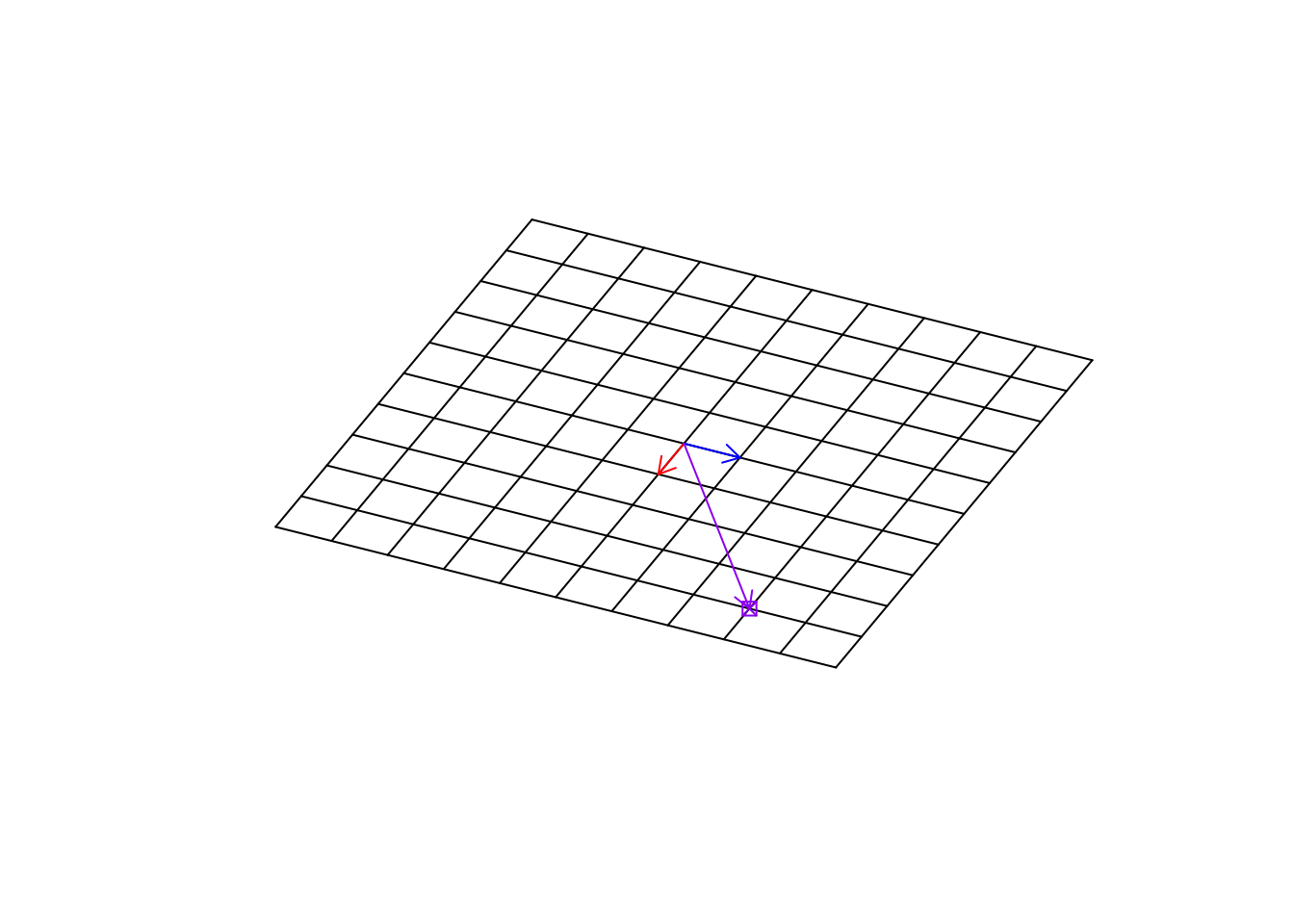
Figure 6.29: Location of the target point in rotation
Exactly! This transformation has rotated our space. It’s really cool. The next time you use software to rotate your picture, you know there is the math behind it!! So, We can change our empty base space to “any space” and still find the location at any point in that space.
Definition 6.9 (Matrix multiplication) Matrix multiplication is used to transform the space into another shape. This multiplication is defined between two matrices and will produce another matrix as the result. In order to be able to multiply two matrices, the number of columns of the first matrix (left-hand side) MUST matches the number of rows in the second matrix. If the dimensions of the first matrix are \(l \times m\) and the dimensions of the second matrix is \(m \times n\), the result of the multiplication will be a matrix with dimensions of \(l \times n\). We show matrix multiplication by just putting to matrix next to each other (e.g. \(AB\) for multiplying \(A\) and \(B\)). Also please remember that \(AB\) is not equal to \(BA\).
To multiply two matrices \(A\) and \(B\), giving \(C\), we take the first row of \(A\) and the first column of \(B\), multiple the corresponding elements, and sum the results. This result will be the first element in \(C\) with location \([1,1]\). We then proceed with the second column of \(B\) matrix and calculate its multiplication with the first row of \(A\), sum the results in \(C\) at the first row and second column [1,2]. We repeat this until all columns of the second matrix have covered. We then move to the second row of \(A\), we repeat this process but put the results in the second row of \(C\). We keep doing this until we multiply all rows of \(A\) by all columns of \(B\).
\[\begin{bmatrix} a & b \\ c & d \end{bmatrix} \ \begin{bmatrix} e & f & g\\ h & i & j \end{bmatrix}=\begin{bmatrix} a \times e + b \times h& a \times f + b \times i & a \times g + b \times j\\ c \times e + d \times h& c \times f + d \times i & c \times g + d \times j \end{bmatrix}\]
Example: \[ \begin{bmatrix} 1 & 2 \\ 4 & 5 \end{bmatrix} \ \begin{bmatrix} 7 & 8 & 9\\ 10 & 11 & 12 \end{bmatrix}=\begin{bmatrix} 1 \times 7 + 2 \times 10& 1 \times 8 + 2 \times 11 & 1 \times 9 + 2 \times 12\\ 4 \times 7 + 5 \times 10& 4 \times 8 + 5 \times 11 & 4 \times 9 + 5 \times 12 \end{bmatrix}=\\\begin{bmatrix} 27 & 30 & 33\\ 78 & 87 & 96 \end{bmatrix} \]
Don’t worry if it’s too much work. You can calculate this with pretty much any statistical software. There are even websites that can help you understand and do this multiplication. But for now, let’s discuss what this matrix multiplication means, in the context of our gene expression dataset.
Considering what we have been saying, do you think our gene expression dataset changes the space?
From the linear algebra perspective, yes it does! It might not be that intuitive in the beginning, but if we assume a stem cell as our basis, we then change this stem cell in a way that represents the exact expression pattern found in a sample. We do pretty much the same thing with our spaces/vectors etc. We start with some basis vectors, a raw “meaningless” space (well, maybe biologically), we then change these to show our gene expression space.
So to summarize, we have a raw space (n dimensions) that is defined by a set of unit vectors (e.g. for two dimensions: \(\vec{x}=[1,0]\) and \(\vec{y}={0,1}\)), we then transform this space using our dataset so we are now in our gene expression space.
We do this simply and naively by
data%*%diag(ncol(data))This funny operation (%%)* will do matrix multiplication. Read verbally, take a raw space with the dimensions of my data ncol(data) and transform it into my gene expression space. What are the results of this operation if you do it in R? Well, it’s going to be the exact gene expression data that you started with. So we actually don’t need to do that, mathematically, we almost always assume that our starting basis vectors are \(\vec{x}=[1,0]\) and \(\vec{y}={0,1}\), etc. So we are in the gene expression space already from the start. Any location/observation/vectors can be found using the combination of genes.
There are a few important things to know before moving forward:
- Each matrix has two spaces: column space and row space
I guess by now, you realized that matrices are very powerful, we can do a lot with them. The question is that what can we say about the transformation a matrix does to our space? If we have thousands of variables (thousands of dimensions), defining our space transformation, it’s difficult to every time plot and sees what it does. We need to be able to at least say something about the transformation without plotting so many arrows and other stuff!
Almost all the operations that we will be talking about in the rest of the chapter is around square matrices. Let’s quickly define them and go forward with the rest of the chapter.
6.4.2 Square matrices
A Square matrix is a matrix with the same number of rows and columns. Square matrices are used in linear algebra quite a lot and are easier to work with. There are several reasons why we want to use square matrices but to summarize all: When we multiply a matrix with \(n\) number of rows and \(m\) number columns by another matrix with \(m\) rows and \(l\) columns, we are mapping the space from \(m\) to \(n\) which is essentially another space which might change the definitions of certain things. In many cases, we would like to stay in the same dimensions (not going to a totally different space). In these cases, square matrices are used to map from \(n\) to \(n\), meaning that it maps from a space to itself. Please note that we are still doing the transformation to the vectors and everything else in that space, but we are in the same dimensions. Let’s look at an example.
par(mfrow=c(2,2))

# load cat data
cat_data<-read.table("data/cat.tsv")
#plot
scatterplot3d::scatterplot3d(cat_data,angle = 150,xlab="",ylab="",zlab = "")
title("Original data")


# rotation matrix
tet<-3.2
b<-matrix(c(1,0,0,0,cos(tet),sin(tet),0,-sin(tet),cos(tet)),nrow = 3,byrow = T)
#plot
scatterplot3d::scatterplot3d(t(b%*%t(as.matrix(cat_data))),xlab="",ylab="",zlab = "")
title("Square matrix (rotation)")


plot(t(b[-1,]%*%t(as.matrix(cat_data))),xlab="",ylab="")
title("2d matrix transformation")

plot(x=t(b[-c(1,2),]%*%t(as.matrix(cat_data))),y=rep(1,nrow(cat_data)),xlab="",ylab="")
title("1d matrix transformation")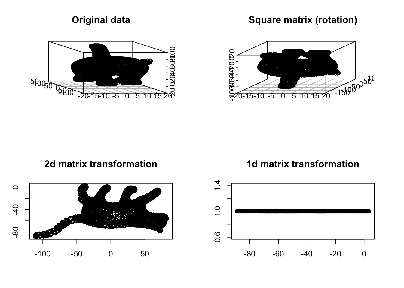
Figure 6.30: Cat example
You see in Figure 6.30 that at some point the meaning of things starts vanishing. We have volume in both top panel but no volume in the bottom ones. Obviously, the 1d transformation totally distorts our view. Can we say the cat’s tail is located in the middle of the body or the legs are almost parallel? Probably not in the 2d and 1d transformation. In any transformation, it’s nice to have the same geometric meaning of the concepts before and after performing such transformation.
In addition, working on square matrices gives us some extra tools that are handy for describing the space and the transformation itself.
6.4.3 Determinant of a matrix
As we discussed before, matrix multiplication will change the space and anything inside. This change can be rotation, stretching, squeezing, etc. Some transformation such squeezing will make the space smaller, some like stretching will make it bigger, and some like rotation does not change the size or the volume of our space. The determinant of a matrix will summarize for us whether the transformation makes the volume of our data smaller or bigger or unchanged. Let’s have a look at an example:
# set number of figures
par(mfrow=c(2,2))

# read the data
cat_data<-read.table("data/cat.tsv")[,2:3]

# plot the original space
plot(cat_data,xlab="",ylab="",xlim=c(-110,110),ylim=c(-150,150))
# write title
title("Original")

# create a rotation matrix
tet<-2
b<-matrix(c(cos(tet),sin(tet),-sin(tet),cos(tet)),nrow = 2,byrow = T)

# plot the rotated data
rt_data<-t(b%*%t(as.matrix(cat_data)))
plot(rt_data,xlab="",ylab="",xlim=c(-110,110),ylim=c(-150,150))
title("Rotated")
# do inverse
bs<-matrix(c(0.5,0,0,0.5),2)
# plot inverse
plot(t(bs%*%t(as.matrix(cat_data))),xlab="",ylab="",xlim=c(-110,110),ylim=c(-150,150))
# write title
title("Squeezing")

bs2<-matrix(c(1.5,0,0,1.5),2)
# plot inverse
plot(t(bs2%*%t(as.matrix(cat_data))),xlab="",ylab="",xlim=c(-110,110),ylim=c(-150,150))
# write title
title("Stretching")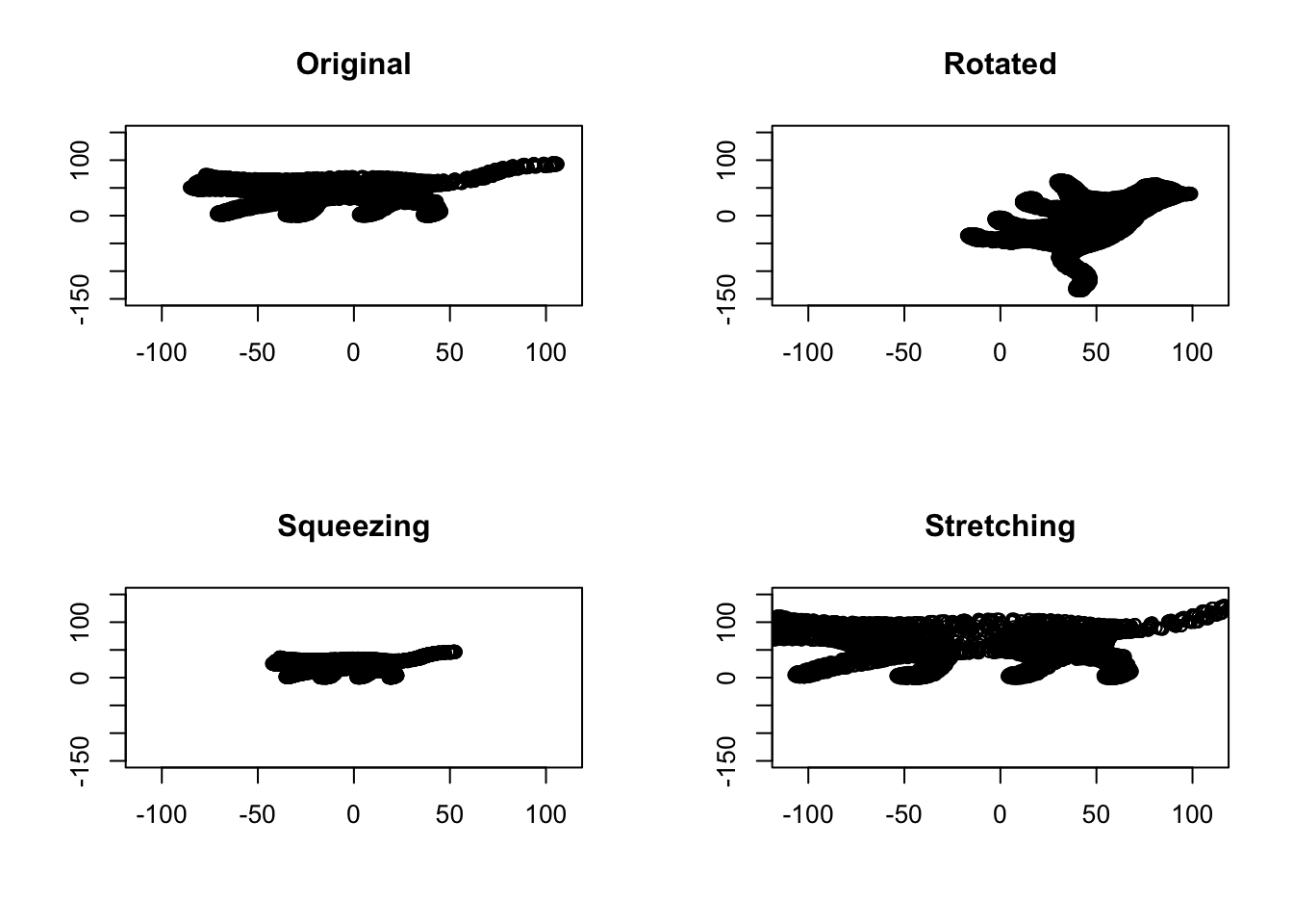
Figure 6.31: Space volume of cat
It’s obvious in Figure 6.32 that, the volume of data is the same between the original cat picture and the rotated one. This gives us a determinant of 1 for rotated space, meaning that the volume has not changed. Anything lower than one means the volume has decreased. For example, in Squeezing, the determinant is 0.25. Obviously, in stretching, the volume has increasing which gives us the determinant of 2.25, meaning that the volume has increased by 2.25 scaling factor.
Definition 6.10 (Determinant) The determinant is a scalar value that is computed from square matrices. The absolute value of the determinant shows the scaling of the volume resulted from the matrix transformation. Here we show the determinant of matrix A by |A|. It should be clear by now that the determinant of zero means that our transformation has mapped the space to something that has no volume, for example, either a line or just the origin. More formally, if there exist two columns or rows in the matrix that are linear dependent (eg. \(\vec{a}=c \times \vec{b}\)), the determinant will be zero.
The determinant of 2 by 2 matrix is calculated by:
\[|A|=\begin{vmatrix} a & b \\ c & d \end{vmatrix}= ad-bc\]
For 3 by 3:
\[|A|=\begin{vmatrix} a & b &c \\ d & e & f\\g & h &i \end{vmatrix}= a\begin{vmatrix} e & f \\ h & i \end{vmatrix}-b\begin{vmatrix} d & f \\ g & i \end{vmatrix}+c\begin{vmatrix} d & e \\ h & g \end{vmatrix}= aei+bfg+cdh-ceg-bdi-afh\]
For example:
\[|A|=\begin{vmatrix} 1 & 0\\ 0 & 1 \end{vmatrix}= 1 \times 1-0 \times 0=1\]
In practice, these numbers are calculated by software for a programming language.
6.4.4 Inverse of a matrix
The inverse of a matrix is defined as the opposite transformation of what it does to space (the inverse of a matrix \(X\) is shown by \(X^{-1}\)). For example, if a matrix rotates the space by \(45^o\), the inverse of it will rotate the space back by \(45^o\). Let’s have a look at an example:
# set number of figures
par(mfrow=c(1,3))

# read the data
cat_data<-read.table("data/cat.tsv")[,2:3]

# plot the original space
plot(cat_data,xlab="",ylab="")
# write title
title("Original space")

# create a rotation matrix
tet<-2
b<-matrix(c(cos(tet),sin(tet),-sin(tet),cos(tet)),nrow = 2,byrow = T)

# plot the rotated data
rt_data<-t(b%*%t(as.matrix(cat_data)))
plot(rt_data,xlab="",ylab="")
title("Rotated data")
# do inverse
bin<-solve(b)
# plot inverse
plot(t(bin%*%t(as.matrix(rt_data))),xlab="",ylab="")
# write title
title("Inverse of rotation")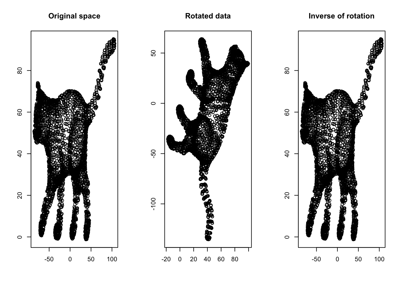
Figure 6.32: Inverse of a matrix
Another way of understanding the inverse is by thinking about division. If we have a scalar \(7\) and multiply it by another scalar \(2\), giving us \(14\), how do we go back to \(2\)? Well, we divide \(14\) by \(7\). The division is matrix world is by multiply the result matrix by the inverse of the transformation matrix. Therefore, we can deduce that if \(\frac{7}{7}=1\), \(X\ X^{-1}=I\). Here \(I\) is a special matrix (called identity matrix) that has “1” on its main diagonal elements and zero elsewhere. I identity matrix does not change the space if multiply with another matrix.
Definition 6.11 (Inverse of a matrix) The inverse of matrix \(A\) is defined by the reverse transformation induced by A which is denoted by \(A^-1\). More formally if the matrix is invertible, there exists another matrix \(A^-1\) where \(A \ A^{-1} =A^{-1} \ A=I\), where \(I\) is identity matrix. Not all the matrices have an inverse. If the determinant (6.10) of a matrix is zero, the matrix is not invertible (there is no reverse transformation).
There are many methods for finding the inverse of a matrix. Here we focus on one solution.
Given, a matrix \(A\), \(A^{-1}\) can be calculated using:
\[A^{-1}=\frac{1}{|A|}\begin{vmatrix} C_{11} & C_{21} & ... & C_{n1}\\ C_{12} & C_{22} & ... & C_{n2}\\.&.&.&.\\.&.&.&.\\.&.&.&.\\C_{1n} & C_{2n} & ... & C_{nn}\ \end{vmatrix}\]
Yes. It looks scary and in fact, it is!. Let’s break it down to three steps:
Step 1: In step one, we want to find that big matrix.
\[\begin{vmatrix} C_{11} & C_{21} & ... & C_{n1}\\ C_{12} & C_{22} & ... & C_{n2}\\\vdots &\vdots&\ddots& \vdots\\C_{1n} & C_{2n} & ... & C_{nn}\ \end{vmatrix}\]
This is called cofactors. It still looks scary but let’s look at the square matrix together.
\[\begin{vmatrix} a & b &c \\ d & e & f\\g & h &i \end{vmatrix}\] Can we see any sub-square in this matrix? Let’s try to see how we can extract the sub squares of this matrix:
Let’s select the first element of the matrix, that is \(a\):
\[\left|\begin{array}{ccc} \textbf{a} & \underline{b} & \underline{c}\\ \underline{d} & \begin{array}{|c} \hline e \end{array} & \begin{array}{c|} \hline f \end{array} \\ \underline{g} & \begin{array}{|c} h\\ \hline \end{array} & \begin{array}{c|} i\\ \hline \end{array}\end{array}\right|\]
\(a\) is bold in the matrix above, if we ignore all elements (underlined text) sitting on the same row (\(b\) and \(c\)) and same column (\(d\) and \(g\)) as \(a\), the rest of the elements give us a square. We just calculate the determinant of this square and call it \(a_t\). We put \(a_t\) in an empty matrix in the exact location of \(a\), \(\begin{vmatrix} a_t & & \\ & & \\ & & \end{vmatrix}\) We now move to the second element in our matrix (\(b\)).
\[\left|\begin{array}{ccc} \underline{a} & \textbf{b} & \underline{c}\\ \begin{array}{|c} \hline d \end{array} & \underline{e} & \begin{array}{c|} \hline f \end{array} \\ \begin{array}{|c} g \\ \hline \end{array} & \begin{array}{c} \underline{h}\\ \end{array} & \begin{array}{c|} i\\ \hline \end{array}\end{array}\right|\]
In this case, if we ignore all the underlined elements, we will end up with another square \(\begin{vmatrix} d & f \\ g & i \end{vmatrix}\), we calculate its determinant call it \(b_t\). We put it in the matrix: \(\begin{vmatrix} a_t & b_t & \\ & & \\ & & \end{vmatrix}\) If we do the same procedure for all the elements of the matrix, we end up with
\[M=\begin{vmatrix} a_t & b_t &c_t \\ d_t & e_t & f_t\\g_t & h_t &i_t \end{vmatrix}\]
This is our matrix of minor.
Step 2
We can now calculate our matrix of cofactors easily. We start from the first element of \(M\) and multiply with \(+1\)
\[M_1=\begin{vmatrix} a_t \times +1 & b_t &c_t \\ d_t & e_t & f_t\\g_t & h_t &i_t \end{vmatrix}\] We now take the second element and multiply by -1!
\[M_1=\begin{vmatrix} a_t \times +1 & b_t \times -1 &c_t \\ d_t & e_t & f_t\\g_t & h_t &i_t \end{vmatrix}\] Now for the third one +1! \[M_1=\begin{vmatrix} a_t \times +1 & b_t \times -1 &c_t \times +1 \\ d_t & e_t & f_t\\g_t & h_t &i_t \end{vmatrix}\] We just keep doing this for all the elements and every time change the sign of \(1\) to \(+\) or \(-\).
\[C=\begin{vmatrix} a_t \times +1 & b_t \times -1 &c_t \times +1 \\ d_t \times -1 & e_t \times +1 & f_t \times -1\\g_t \times +1 & h_t \times -1 &i_t\times +1 \end{vmatrix}\] We now transpose \(C\).
Definition 6.12 (Transpose of a matrix) Transpose of a matrix is simply an operation and swap the position of rows and columns of the matrix, so the first column of the matrix is now the first row and so forth. Transpose of matrix \(X\) is shown by \(X^T\). For example,
\(X=\begin{vmatrix} a & b &c \\ d & e & f\\g & h &i \end{vmatrix}\) So
\(X^{T}=\begin{vmatrix} a & d &g \\ b & e & h\\c & f &i \end{vmatrix}\)At this stage, the big formula we had up there can be written as \[A^{-1}=\frac{1}{|A|}C^T\] Where \(C^T\) is the transpose of the \(C\) matrix we calculate up there and \(|A|\) is determinant of \(A\) that we know how to calculate (6.10).
For example,
\[A=\begin{vmatrix} 1 & 4 & 3\\ 1 & 5 & 1\\ 3 & 2 & 1\\ \end{vmatrix}\]
We find \(a_t=5 \times 1 - 1 \times 2=3\), \(b_t=1 \times 1 - 1 \times 3=-2\), … , \(i_t=1 \times 5 - 4 \times 1=1\)
We put them to a matrix
\[C= \begin{vmatrix} 3 & -2 & -13\\ -2 & -8 & -10\\ -11 & -2 & 1\\ \end{vmatrix}\]
Now we multiply this by \(+\) and \(-\) (this is elementwise multiplication: each element on the left-hand matrix will be multiplied by its corresponding one right hand):
\[C=\begin{vmatrix} 3 & -2 & -13\\ -2 & -8 & -10\\ -11 & -2 & 1\\ \end{vmatrix} \times \begin{vmatrix} 1 & -1 & 1\\ -1 & 1 & -1\\ 1 & -1 & 1\\ \end{vmatrix}=\begin{vmatrix} 3 & 2 & -13\\ 2 & -8 & 10\\ -11 & 2 & 1\\ \end{vmatrix}\]
we can now calculate the transpose of \(C\):
\[C^T=\begin{vmatrix} 3 & 2 & -13\\ 2 & -8 & 10\\ -11 & 2 & 1\\ \end{vmatrix}^{T}=\begin{vmatrix} 3 & 2 & -11\\ 2 & -8 & 2\\ -13 & 10 & 1\\ \end{vmatrix}\]
So
\[A^{-1}=\frac{1}{|A|}C^T= \frac{1}{-28} \begin{vmatrix} 3 & 2 & -11\\ 2 & -8 & 2\\ -13 & 10 & 1\\ \end{vmatrix}=\begin{vmatrix} -0.1071429 & -0.0714286 & 0.3928571\\ -0.0714286 & 0.2857143 & -0.0714286\\ 0.4642857 & -0.3571429 & -0.0357143\\ \end{vmatrix} \]
In practice you will use a function in R to do that:
solve(A)Easy right?! Let’s move forward.
6.4.5 Rank of a matrix
Remember we talked about the basis vectors (6.8)? We said that the basis vectors are vectors that define our space and they must be linearly independent. The linear independence means that, if we select one of the basis vectors, this vector cannot be constructed by linearly combining the other vectors. For example we consider our standard basis vectors in 3d dimensions \(\vec{x}=[1,0,0]\), \(\vec{y}=[0,1,0]\), and \(\vec{z}=[0,0,1]\), Can we come us with a formula to combine \(\vec{x}\) and \(\vec{y}\) to be equal to \(\vec{z}\)? We said that we can use addition, multiplication, subtraction, etc. For example, can we find a scalar \(c\) such that \(\vec{z}=c \times \vec{x} + c \times \vec{y}\)? The answer is no if the vectors are linearly independent. By definition, the standard basis vectors are linearly independent. But here comes a problem! We said a matrix will change our space including the position of our standard basis vectors. So are these new locations (vectors) linearly independent? Or similarly, can the new vectors be called basis vectors? Let’s have a look at an example:
# fix the plot number
par(mfrow=c(1,1))

# create basis vector
basis_vectors<-matrix(c(1,0,0,1),byrow = T,nrow = 2)

# create transformation matrix
b<-matrix(c(1,2,3,6),nrow = 2,byrow = T)

# create the transformed vectors
trasformed_spcae<-b%*%basis_vectors

# empty plot
plot(c(0,11),c(0,11),type="n",xlab = "",ylab="")


## base arrows
# arrows
arrows(0,0,1,0,col="blue")
# arrows
arrows(0,0,0,1,col="red")


# trasformed arrows
# arrows
arrows(0,0,trasformed_spcae[1,1],trasformed_spcae[2,1],col="blue",lty = "dashed")
# arrows
arrows(0,0,trasformed_spcae[1,2],trasformed_spcae[2,2],col="red",lty="dashed")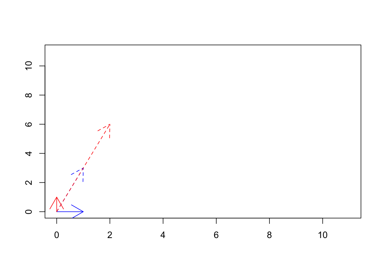
Figure 6.33: The transformed basis vectors
We see if Figure 6.33 that using \(\begin{vmatrix} 1&2\\3&6 \end{vmatrix}\) matrix we transformed our basis vectors from \(\vec{x}=[1,0] \ and \ \vec{y}=[0,1]\) (solid lines) to \(\vec{x}=[1,3] \ and \ \vec{y}=[2,6]\). Are these new vectors basis vectors? We can see that \(\vec{y}\) is basically \(2 \times \vec{x}\), so no they are not basis vectors. In fact, they might be thought of as redundant. Thinking about addressing in space, we can go to exact locations that we can go with \(\vec{y}\) using \(\vec{x}\). So all of these means that we have only one basis vector in the new space! This is related to the rank of a matrix.
There many methods for calculating the rank of a matrix. The simplest one is called row reduction or even fancier Gaussian elimination! Without going into much detail about this beast, this is a process by which would like to transform our matrix into a form where everything becomes zero! Well, that sounds easy! We can just multiply a matrix by zero! Nope! We are given three tools:
- 1: We can only multiply a row by a non zero scalar
- 2: We can swap the position of two rows
- 3: We can add or subtract two rows from each other
We can use any number of steps above in order to reach our goal. We at some stage, it was not possible to go forward, we just stop. We count the number of non-zero rows, that is the rank of the matrix! Let’s start with
\(A=\begin{vmatrix} 1&2&3\\4&5&12\\3&1&9\end{vmatrix}\)
Let’s for the start, add “4” to the first row
\[\begin{vmatrix} 4&8&12\\4&5&12\\3&1&9\end{vmatrix}\] Why did we add 4? Because we looked at the first and third entities of the second row and saw it’s like that first row multiply by 4! Doing that will give us the chance of subtracting the first row from the second one making some elements zero! Let’s do it.
\[\begin{vmatrix} 4&8&12\\0&-3&0\\3&1&9\end{vmatrix}\]
Awww! We are getting close. Now let’s do the same thing for the third row!
Now multiply the first row by \(\frac{3}{4}\)
\[\begin{vmatrix} 3&6&9\\0&-3&0\\3&1&9\end{vmatrix}\]
Then subtract from the third row.
\[\begin{vmatrix} 3&6&9\\0&-3&0\\0&-5&0\end{vmatrix}\]
A little bit more! We multiply the second row with \(\frac{5}{3}\)
\[\begin{vmatrix} 3&6&9\\0&-5&0\\0&-5&0\end{vmatrix}\] You see, now we can get rid of the third row by subtracting the second row from the third one!
\[\begin{vmatrix} 3&6&9\\0&-5&0\\0&0&0\end{vmatrix}\] At this point, no matter how much we try, we won’t be able to change make the first and the second row zero. What is the rank of the matrix? It’s the number of non zero rows. That is 2!
In practice, you can calculate that using a function in R (like this one in Matrix package):
Matrix::rankMatrix()We are now ready to know a bit more about the matrices. Let’s move forward to one of the most amazing topics linear algebra.
6.4.6 Eigenvector & eigenvalues
Remember, we said if we multiply a matrix \(A\) by \(B\) (\(A\ B\)), it will transform the space of \(B\) including all the vectors inside B?
par(mfrow=c(1,2))


# data
mydata<-cbind(-5:5,rep(-5,11),-5:5,rep(5,11))

mydata2<-cbind(rep(-5,11),-5:5,rep(5,11),-5:5)
# plot
plot(range(rbind(mydata[,1],mydata[,3])),range(rbind(mydata[,2],mydata[,4])),
     type="n",xlab="",ylab="",xlim=c(-5,5),ylim=c(-5,5),axes = F,bg="black")

# lines
nl<-apply(mydata,MARGIN = 1,function(x){
  segments(x[1],x[2],x[3],x[4],col = "grey")})

nl<-apply(mydata2,MARGIN = 1,function(x){
  segments(x[1],x[2],x[3],x[4],col = "grey")})


arrows(0,0,1,0,col="red",length=0.1)
arrows(0,0,0,1,col="blue",length=0.1)
title("Original space")

# another data
mydata<-cbind(-5:5,rep(-5,11),-5:5,rep(5,11))

mydata2<-cbind(rep(-5,11),-5:5,rep(5,11),-5:5)
# plot
plot(range(rbind(mydata[,1],mydata[,3])),range(rbind(mydata[,2],mydata[,4])),
     type="n",xlab="",ylab="",xlim=c(-8,8),ylim=c(-8,8),axes = F,bg="black")

# transformation matrix
b<-as.matrix(data.frame(a=c(1,0),b=c(1,2)))
# multiplication
mydata[,c(1,2)]<-t(b%*%t(mydata[,c(1,2)]))
mydata[,c(3,4)]<-t(b%*%t(mydata[,c(3,4)]))

mydata2[,c(1,2)]<-t(b%*%t(mydata2[,c(1,2)]))
mydata2[,c(3,4)]<-t(b%*%t(mydata2[,c(3,4)]))
# lines
nl<-apply(mydata,MARGIN = 1,function(x){
  segments(x[1],x[2],x[3],x[4],col = "grey")})

nl<-apply(mydata2,MARGIN = 1,function(x){
  segments(x[1],x[2],x[3],x[4],col = "grey")})
# arrows
arrows(0,0,1,0,col="red",length=0.1,)
arrows(0,0,1,2,col="blue",length=0.1)
title("Transformed space")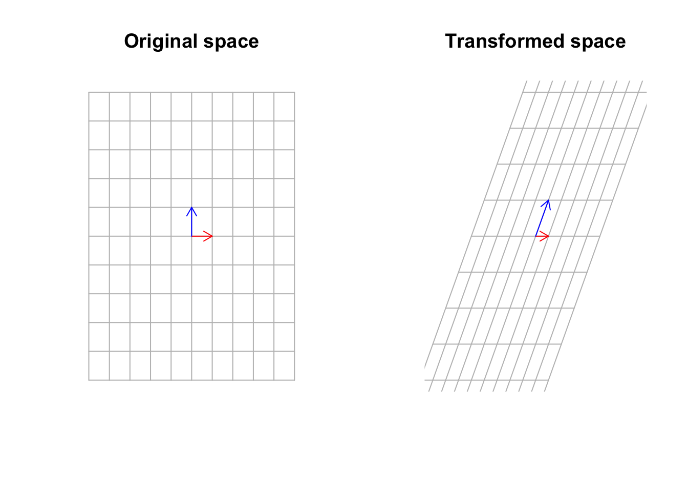
Figure 6.34: Multiply a matrix to space, including the basis vectors
Well, yes that’s true but not completely true! Sometimes there exist some vectors that the matrix transformation cannot move that much! In fact, it can move them by just stretching them. It cannot move the span of those vectors.
par(mfrow=c(1,2))


# data
mydata<-cbind(-5:5,rep(-5,11),-5:5,rep(5,11))

mydata2<-cbind(rep(-5,11),-5:5,rep(5,11),-5:5)
# plot
plot(range(rbind(mydata[,1],mydata[,3])),range(rbind(mydata[,2],mydata[,4])),
     type="n",xlab="",ylab="",xlim=c(-5,5),ylim=c(-5,5),axes = F,bg="black")

# lines
nl<-apply(mydata,MARGIN = 1,function(x){
  segments(x[1],x[2],x[3],x[4],col = "grey")})

nl<-apply(mydata2,MARGIN = 1,function(x){
  segments(x[1],x[2],x[3],x[4],col = "grey")})


arrows(0,0,1,0,col="red",length=0.1)
arrows(0,0,0,1,col="blue",length=0.1)


arrows(0,0,eigen(b)$vectors[1,1],eigen(b)$vectors[2,1],col="purple",length=0.1)
segments(-10,-10,eigen(b)$vectors[1,1]*10,eigen(b)$vectors[2,1]*10)

title("Original space")

# send data
mydata<-cbind(-5:5,rep(-5,11),-5:5,rep(5,11))

mydata2<-cbind(rep(-5,11),-5:5,rep(5,11),-5:5)

plot(range(rbind(mydata[,1],mydata[,3])),range(rbind(mydata[,2],mydata[,4])),
     type="n",xlab="",ylab="",xlim=c(-8,8),ylim=c(-8,8),axes = F,bg="black")

# matrix transformation
b<-as.matrix(data.frame(a=c(1,0),b=c(1,2)))

mydata<-cbind(-5:5,rep(-5,11),-5:5,rep(5,11))

mydata2<-cbind(rep(-5,11),-5:5,rep(5,11),-5:5)
# do the transform
mydata[,c(1,2)]<-t(b%*%t(mydata[,c(1,2)]))
mydata[,c(3,4)]<-t(b%*%t(mydata[,c(3,4)]))

mydata2[,c(1,2)]<-t(b%*%t(mydata2[,c(1,2)]))
mydata2[,c(3,4)]<-t(b%*%t(mydata2[,c(3,4)]))
# lines and arrows
nl<-apply(mydata,MARGIN = 1,function(x){
  segments(x[1],x[2],x[3],x[4],col = "grey")})

nl<-apply(mydata2,MARGIN = 1,function(x){
  segments(x[1],x[2],x[3],x[4],col = "grey")})

arrows(0,0,1,0,col="red",length=0.1,)
arrows(0,0,1,2,col="blue",length=0.1)

arrows(0,0,(b%*%eigen(b)$vectors)[1,1],(b%*%eigen(b)$vectors)[2,1],col="purple",length=0.1)
segments(-10,-10,(b%*%eigen(b)$vectors)[1,1]*10,(b%*%eigen(b)$vectors)[2,1]*10)

title("Transformed space")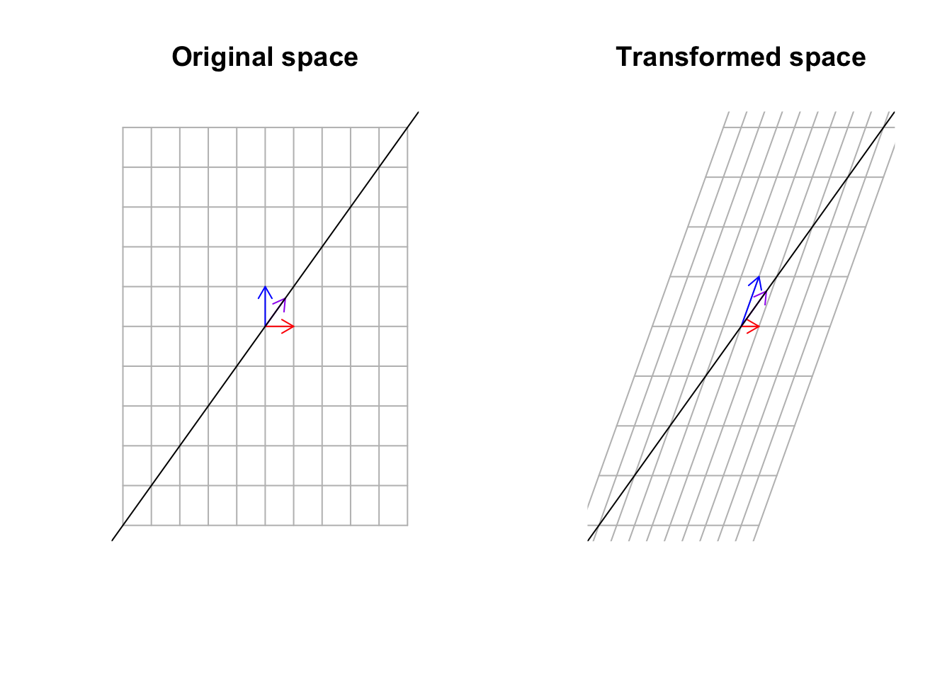
Figure 6.35: Multiply a matrix to space, including the basis vectors and span of eigen vectors
What we see in Figure 6.35 is that the purple vector stays on its span (the black line) but the blue vector has been knocked off its span. These vectors that stay on their span might be stretched or flipped but they will hold on to the span. Can you find another vector that stays on its span? Yes exactly. That is the red one! It is the same vector, the same size, and the same direction. These guys are called eigenvectors. Pretty awesome, right!? But we said although the vector stays on its span can be stretched. How much? The value that this specific vector is stretched by is called an eigenvalue. I agree! That is difficult to imagine! Let’s look at our cat!
par(mfrow=c(1,1))
# read data
cat_data<-read.table("data/cat.tsv")[,2:3]
# center
cat_data<-scale(cat_data,center = T)
# plot
plot(cat_data,xlab="",ylab="",xlim=c(-5,5),ylim=c(-5,5))
title("Original cat image")


# transoform
b<-as.matrix(data.frame(a=c(1,10),b=c(1,2)))

# plot eigens
arrows(eigen(b)$vectors[1,1]*100,eigen(b)$vectors[2,1]*100,eigen(b)$vectors[1,1]*-100,eigen(b)$vectors[2,1]*-100,col="blue",length=0.1)

arrows(eigen(b)$vectors[1,2]*-100,eigen(b)$vectors[2,2]*-100,eigen(b)$vectors[1,2]*100,eigen(b)$vectors[2,2]*100,col="red",length=0.1)


# plot selected points
eigenB<-eigen(b)
eigendif<-apply(cat_data,1,function(x){data.frame(x=x[1]/eigenB$vectors[1,1],y=x[2]/eigenB$vectors[2,1])})

for(x in which(abs(unlist(sapply(eigendif,function(x){x[1]-x[2]})))<0.2))
{
  points(cat_data[x][1],cat_data[x,][2],col="green",pch=4)
}


# transformation
eigendif<-apply(cat_data,1,function(x){data.frame(x=x[1]/eigenB$vectors[1,2],y=x[2]/eigenB$vectors[2,2])})

# plot
selectedPoints2<-which(abs(unlist(sapply(eigendif,function(x){x[1]-x[2]})))<0.1)
for(x in selectedPoints2)
{
  points(cat_data[x][1],cat_data[x,][2],col="purple",pch=4)
}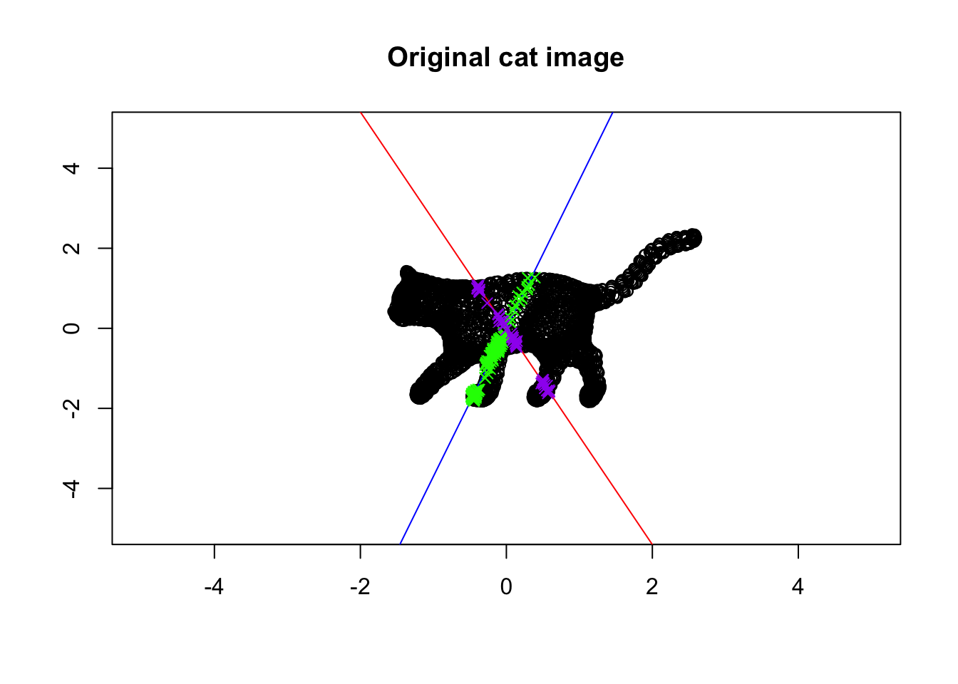
Figure 6.36: Eigenvector and values of a cat!
In this Figure, we plotted the eigenvectors of the cat! The blue one is the eigenvector with the largest span of eigenvalue whereas the red line is the span of the eigenvector with the smallest eigenvalue. There are some green points also on the plot. These are the points that are colored green and purple. The green points are on (or very close) to the first eigenvector. The purple ones are on the second eigenvector.
Let’s now look at what happens when we transform the space using our amazing matrix:
par(mfrow=c(1,1))
# data
cat_data<-read.table("data/cat.tsv")[,2:3]

cat_data<-scale(cat_data,center = T)

# make transform matrix
b<-as.matrix(data.frame(a=c(1,10),b=c(1,2)))
# do transformation
cat_data<-t(b%*%t(cat_data))
cat_data<-scale(cat_data,center = T)

# Plot
plot(cat_data,xlab="",ylab="",xlim=c(-5,5),ylim=c(-5,5))
title("Transformed cat image")


# map eigens
eigenVectors<-eigen(b)$vectors

eigenVectors<-b%*%eigenVectors


arrows(eigenVectors[1,1]*100,eigenVectors[2,1]*100,eigenVectors[1,1]*-100,eigenVectors[2,1]*-100,col="blue",length=0.1)

arrows(eigenVectors[1,2]*-100,eigenVectors[2,2]*-100,eigenVectors[1,2]*100,eigenVectors[2,2]*100,col="red",length=0.1)


# plot saved points
eigenB<-eigen(b)
eigendif<-apply(cat_data,1,function(x){data.frame(x=x[1]/eigenB$vectors[1,1],y=x[2]/eigenB$vectors[2,1])})

for(x in which(abs(unlist(sapply(eigendif,function(x){x[1]-x[2]})))<0.2))#which(abs(tmp[,1]-tmp[,2])<0.013))
{
  points(cat_data[x][1],cat_data[x,][2],col="green",pch=4)
}

# plot saved
eigendif<-apply(cat_data,1,function(x){data.frame(x=x[1]/eigenB$vectors[1,2],y=x[2]/eigenB$vectors[2,2])})

selectedPoints2<-which(abs(unlist(sapply(eigendif,function(x){x[1]-x[2]})))<0.1)
for(x in selectedPoints2)#which(abs(tmp[,1]-tmp[,2])<0.013))
{
  points(cat_data[x][1],cat_data[x,][2],col="purple",pch=4)
}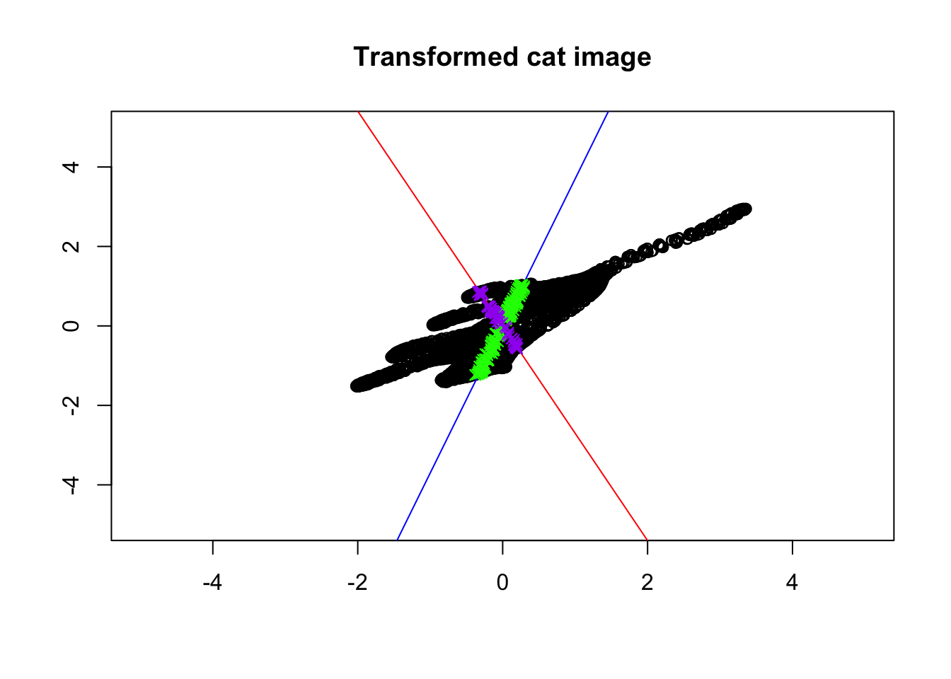
Figure 6.37: Eigenvector and values of transformed cat!
Isn’t this beautiful? The colored points are still on the same lines! Every other point (black ones) have changed directions. Put it simply, the eigenvectors give us the direction which does not change direction after transforming the data. In other words, it gives us the axis around which our image has been transformed. That is the reason why the points on the eigenvectors will never go off their spans. Let’s take it step by step! First, consider the blue line. We took the blue line and then flipped the cat around the blue line. We then did some stretching. Next, we took the red line and did a bit of squeezing. So great. So we now know the axis of rotation. But how about squeezing and stretching? It seems like the distance between the head and the tip of the tails of the cat is a bit longer in Figure 6.37 compared to the original image (6.36). Also, the distance between the feet and the back of the cat seems to be squeezed. Can we say that we actually stretched the cat along the blue line so that the cat is more spread along the blue line? Yes of course. We also did squeezing along the red line so the cat is less spread along that line. The eigenvalues exactly say the same thing! Do you remember, the blue line is the first eigenvector that has the largest eigenvalue, meaning that it has more spread than the red line? The same applies to gene expression data. The eigenvalues can be thought of as the backbone of data or its structure (you will see soon). The eigenvalues are spread of the data on these lines. So now we have tools to find the spread of our space (e.g. variance) and also we know in which direction space has been changed. But there might still be a question that: why are these vectors are so important for us? Well, simply talking we can use these vectors to squish the whole space into a single line. But this line has a very specific meaning, that the direction of changes our data has done to space which in turn means the direction in which our data has the most variance. These directions can be used to define another space that can be thought of as a backbone of our data. Let’s look at an example.
Imagine we have a matrix of \[A=\begin{vmatrix} 2&1\\7&2\end{vmatrix}\] You can consider this as a very small, gene expression data where we have two genes (columns) and two patients (rows) We also want to define our space by basis vector \(\vec{y}=[0,1]\) so \(\vec{x}=[0,0]\) or we just ignore \(x\) for now. What does this transformation look if we do \(A \ y\)? Let’s have a look:
par(mfrow=c(2,2))


# some data
mydata<-cbind(-5:5,rep(-5,11),-5:5,rep(5,11))

mydata2<-cbind(rep(-5,11),-5:5,rep(5,11),-5:5)

# plot
plot(range(rbind(mydata[,1],mydata[,3])),range(rbind(mydata[,2],mydata[,4])),
     type="n",xlab="",ylab="",xlim=c(-8,8),ylim=c(-8,8),axes = F,bg="black")

# lines
nl<-apply(mydata,MARGIN = 1,function(x){
  segments(x[1],x[2],x[3],x[4],col = "grey")})

nl<-apply(mydata2,MARGIN = 1,function(x){
  segments(x[1],x[2],x[3],x[4],col = "grey")})

# arrows
arrows(0,0,1,0,col="red",length=0.1)
arrows(0,0,0,1,col="blue",length=0.1)

title("Original space")

# another set
mydata<-cbind(-5:5,rep(-5,11),-5:5,rep(5,11))

mydata2<-cbind(rep(-5,11),-5:5,rep(5,11),-5:5)

plot(range(rbind(mydata[,1],mydata[,3])),range(rbind(mydata[,2],mydata[,4])),
     type="n",xlab="",ylab="",xlim=c(-8,8),ylim=c(-8,8),axes = F,bg="black")

# transform matrix
b<-as.matrix(data.frame(a=c(2,7),b=c(1,2)))

mydata<-cbind(-5:5,rep(-5,11),-5:5,rep(5,11))

mydata2<-cbind(rep(-5,11),-5:5,rep(5,11),-5:5)
# do transformation
mydata[,c(1,2)]<-t(b%*%t(mydata[,c(1,2)]))
mydata[,c(3,4)]<-t(b%*%t(mydata[,c(3,4)]))

mydata2[,c(1,2)]<-t(b%*%t(mydata2[,c(1,2)]))
mydata2[,c(3,4)]<-t(b%*%t(mydata2[,c(3,4)]))

# plot lines
nl<-apply(mydata,MARGIN = 1,function(x){
  segments(x[1],x[2],x[3],x[4],col = "grey")})

nl<-apply(mydata2,MARGIN = 1,function(x){
  segments(x[1],x[2],x[3],x[4],col = "grey")})

arrows(0,0,b[1,1],b[2,1],col="red",length=0.1,)
arrows(0,0,b[1,2],b[2,2],col="blue",length=0.1)

title("Transformed space")


plot(t(b),xlab="",ylab="",xlim=c(-8,8),ylim=c(-8,8),axes = T,bg="black")
text(t(b),labels = c("sample 1","sample 2"),adj = 1.2)
arrows(0,0,b[1,1],b[2,1],col="red",length=0.1,)
arrows(0,0,b[1,2],b[2,2],col="blue",length=0.1)
title("Transformed space without grid")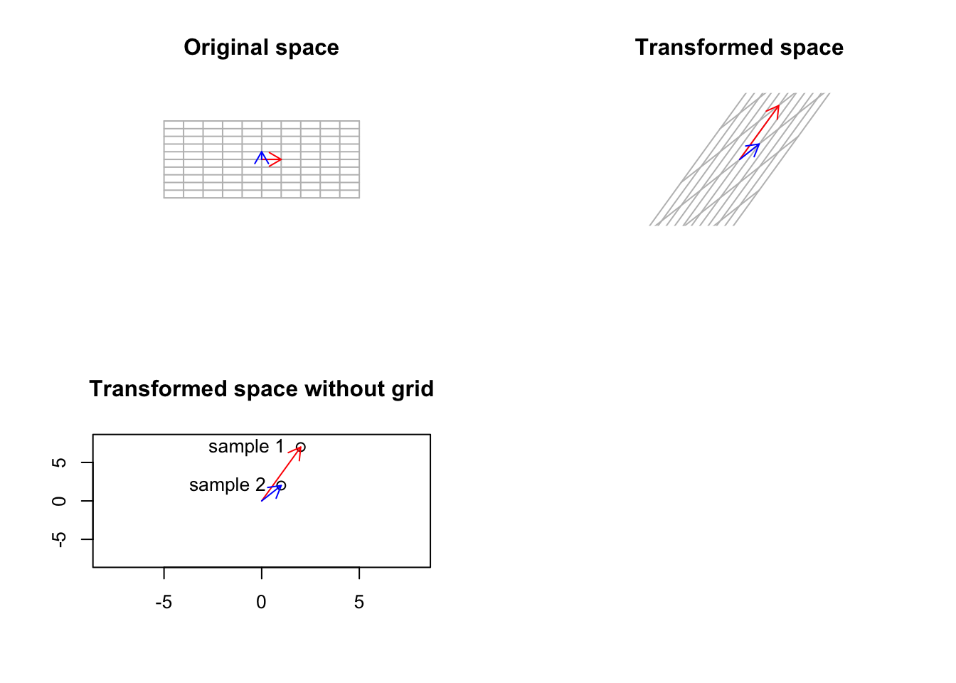
Figure 6.38: Smal gene expression matrix has been used to trasform a basic space
Well, that was not unexpected. As we talked about before, our small gene expression matrix changes the basis vectors to point to each patient. However, as mentioned, it also transformed the base, standard space to the gene expression space. How about if we start from another space which is different from the standard one. Well, we saw that standard space has a simple meaning: a space that can be transformed to anything, and after the transformation, its not the standard space anymore! But do we have another space that has a more concrete meaning compared to the standard one and still keeps its meaning if we transform it? Yes, we do. That is the space defined by our eigenvectors. The eigenvectors cannot be changed (their span of course), so they keep their meaning even after transformation:
par(mfrow=c(2,2))
# transformation matrix
b<-as.matrix(data.frame(a=c(2,7),b=c(1,2)))
# plot
plot(range(rbind(mydata[,1],mydata[,3])),range(rbind(mydata[,2],mydata[,4])),
     type="n",xlab="",ylab="",xlim=c(-5,5),ylim=c(-5,5),axes = T,bg="black")

title("Original eigen space")
# plot eigen lines
eigen_b<-eigen(b)
for(i in -110:110)
{
 abline(a=i,eigen_b$vectors[2,1]/eigen_b$vectors[1,1],col="grey")
 abline(a=i,eigen_b$vectors[2,2]/eigen_b$vectors[1,2],col="grey")
}


# draw arrows and spans
eigen_b$vectors<-eigen_b$vectors

arrows(0,0,eigen_b$vectors[1,1],eigen_b$vectors[2,1],col="red",length=0.1)
text(eigen_b$vectors[1,1],eigen_b$vectors[2,1],"eigen1",adj = -0.5,col = "red")

arrows(0,0,eigen_b$vectors[1,2],eigen_b$vectors[2,2],col="blue",length=0.1)
text(eigen_b$vectors[1,1],eigen_b$vectors[2,1],"eigen2",adj = 2,col = "blue")


segments(0,0,eigen_b$vectors[1,1]*10,eigen_b$vectors[2,1]*10,col="red",lty = "dashed")
segments(0,0,eigen_b$vectors[1,2]*10,eigen_b$vectors[2,2]*10,col="blue",lty = "dashed")

segments(0,0,eigen_b$vectors[1,1]*-10,eigen_b$vectors[2,1]*-10,col="red",lty = "dashed")
segments(0,0,eigen_b$vectors[1,2]*-10,eigen_b$vectors[2,2]*-10,col="blue",lty = "dashed")

# map the eigens to the space
eigen_b$vectors<-b%*%eigen_b$vectors

plot(range(rbind(mydata[,1],mydata[,3])),range(rbind(mydata[,2],mydata[,4])),
     type="n",xlab="",ylab="",xlim=c(-5,5),ylim=c(-5,5),axes = T,bg="black")

# draw spans
for(i in -110:110)
{
 abline(a=i,eigen_b$vectors[2,1]/eigen_b$vectors[1,1],col="grey")
 abline(a=i,eigen_b$vectors[2,2]/eigen_b$vectors[1,2],col="grey")
}

# arrows and other stuff!

arrows(0,0,eigen_b$vectors[1,1],eigen_b$vectors[2,1],col="red",length=0.1)


arrows(0,0,eigen_b$vectors[1,2],eigen_b$vectors[2,2],col="blue",length=0.1)

segments(0,0,eigen_b$vectors[1,1]*10,eigen_b$vectors[2,1]*10,col="red",lty = "dashed")
segments(0,0,eigen_b$vectors[1,2]*10,eigen_b$vectors[2,2]*10,col="blue",lty = "dashed")

segments(0,0,eigen_b$vectors[1,1]*-10,eigen_b$vectors[2,1]*-10,col="red",lty = "dashed")
segments(0,0,eigen_b$vectors[1,2]*-10,eigen_b$vectors[2,2]*-10,col="blue",lty = "dashed")

title("Transformed space")


plot(t(eigen_b$vectors),xlab="",ylab="",xlim=c(-5,5),ylim=c(-5,5),axes = T,bg="black")
text(t(eigen_b$vectors),labels = c("sample 1","sample 2"),adj = 1.2)
arrows(0,0,eigen_b$vectors[1,1],eigen_b$vectors[2,1],col="red",length=0.1,)
arrows(0,0,eigen_b$vectors[1,2],eigen_b$vectors[2,2],col="blue",length=0.1)
title("Transformed space without grid")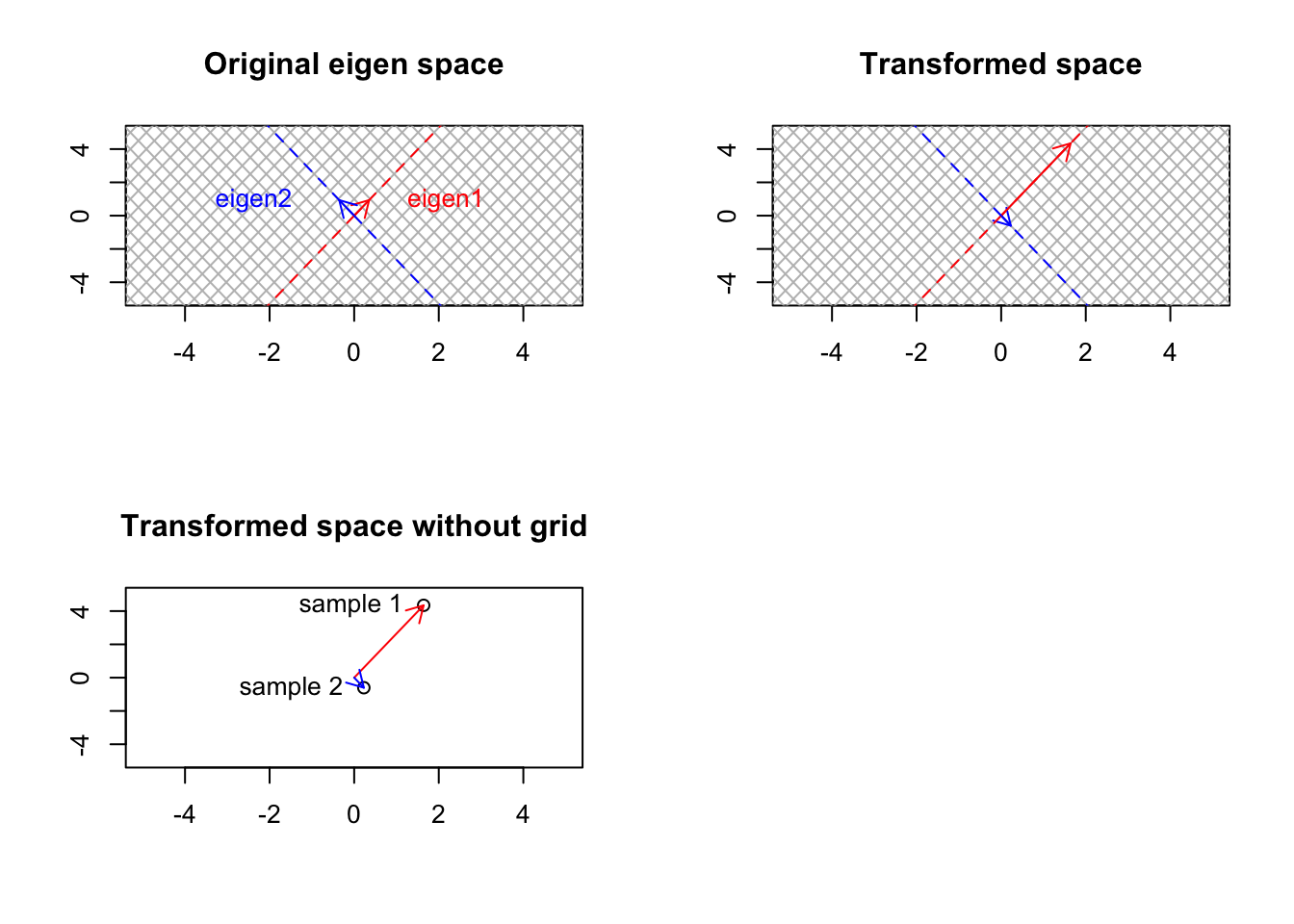
Figure 6.39: Smal gene expression matrix has been used to transform the eigenvector space
What happened? Well, instead of the standard basis, we started from another set of bases (eigenbasis). In Figure 6.39, we plotted the eigenvectors as those small little red and blue vectors. Their corresponding span has been plotted as dashed lines and we have grid lines (line parallel to the vectors). We then did the transformation of \(A \ E\) where \(E\) is now our matrix of eigenvectors. What we see in the upper right panel is that our transformation could not change the space! The eigenvectors were stretched or squeezed but they are on the same spans. What does this mean? Let’s start from the start, we had a basis vector defining a space for us. We took our data, smashed it into that space. Because space was too “flexible”, our data changed the space to the shape of our data. Like smashing an apple to a wall made of dough! It was too flexible! We changed our basis to eigenvectors (concrete wall). We smash our data to this new space so instead of reshaping the wall, our data gets flattened on the space, giving us its overall shape. That is the lower-left panel in Figure 6.39. Another interesting point, if our data is an apple (3d), we smash to dough (standard space), the dough itself is going to be 3d! But if we define a concrete wall (eigenspace) that is 2d and smash our 3d apple against it, the apple is going to be 2d! Yes! This sounds familiar, right? This is dimensionality reduction. Exactly what PCA or similar methods do for us! Fun is enough! Let’s try to mathematically find that concrete wall!
Definition 6.14 (Eigenvectors and eigenvalues) Eigenvectors are vectors in space that when transformed by a matrix, do not change span but only scale by a certain factor. This scaling factor is called an eigenvalue. So if we have eigenvectors in \(v\) and we have a matrix \(A\):
\(A \ v = \lambda \ v\)
Which is basically saying that after transformation, our eigenvectors are just become scaled by \(\lambda\) (which is scalar)! As opposed to what some think, eigenvectors might not necessarily orthogonal to each other. In special cases of symmetric matrix (a matrix that has same things on upper diagonal elements than the lower part (for example, \(A=\begin{vmatrix} 1&2&3\\2&4&6\\3&6&9\end{vmatrix}\)), the eigenvectors become orthogonal. The number of eigenvectors in a matrix is equal to its rank.
How do we calculate the eigenvalues and eigenvectors from this equation? Let’s go step by step.
\(A \ v = \lambda \ v\)
We have a few problems now, \(A\) and \(v\) are matrices but \(\lambda\) is just a number. If we want to solve this funny equation, we have brought \(\lambda \ v\) to the left part of the equation. To do so we have to transform it into a matrix shape by just multiply it to an identity matrix, the size of the number of columns of \(A\). So let’s do it
\(A \ v = \lambda \ I_n \ v\)
We can now safely bring \(\lambda \ I_n \ v\) to the left part.
\(A \ v - \lambda \ I_n \ v=0\)
Noticed how \(v\) is repeating here? We have \(A \ v\) and \(\lambda \ I_n \ v\), we can factor \(v\) and rewrite the whole thing as
\((A -\lambda \ I_n) \ v=0\)
Ok! That became a little boring. To solve this, we could just find the inverse of \((A -\lambda \ I_n)\) and multiply it by both sides? We know that if we multiply a matrix by its inverse, the result will be an identity matrix (like 1 in you divide a number by itself). In this case, \(v\) will be zero. So our eigenvector is just zero! Boring!
Let’s be smart! We have matrix \(A\), that is our data. We are left with one parameter to change that \(\lambda\), we can choose \(\lambda\) in a way that \((A -\lambda \ I_n)\) does not have an inverse anymore so we cannot end up with \(v=0\)! Smart right?
Do you remember when a matrix did not have an inverse (6.10)? Exactly, when its determinant is zero! So we want to find a \(\lambda\) so determinant of \((A -\lambda \ I_n)\) is zero. That is
\(|A -\lambda \ I_n|=0\)
We know \(A=\begin{vmatrix} 2&1\\7&2\end{vmatrix}\) and \(I_n=\begin{vmatrix} 1&0\\0&1\end{vmatrix}\) let’s put back thins:
\(|\begin{vmatrix} 2&1\\7&2\end{vmatrix} -\lambda \ \begin{vmatrix} 1&0\\0&1\end{vmatrix}|=0\)
We know that if we multiply a scalar by a matrix, every element of the matrix will be multiplied by that scalar so what is \(\lambda \ \begin{vmatrix} 1&0\\0&1\end{vmatrix}\)?
It’s
\[\begin{vmatrix} \lambda \times 1 &\lambda \times 0\\ \lambda \times 0 & \lambda \times 1 \end{vmatrix}= \begin{vmatrix} \lambda &0\\0&\lambda \end{vmatrix}\]
Awesome! let’s put back things in \(|\begin{vmatrix} 2&1\\7&2\end{vmatrix} -\lambda \ \begin{vmatrix} 1&0\\0&1\end{vmatrix}|=0\):
\[|\begin{vmatrix} 2&1\\7&2\end{vmatrix} - \begin{vmatrix} \lambda &0\\0&\lambda \end{vmatrix}|=0\]
Let’s move forward! We know that if we subtract two matrices of similar size, each element of the left hand side will be subtracted by the corresponding element of the left hand side. So,
\(|\begin{vmatrix} 2-\lambda&1-0\\7-0 & 2-\lambda\end{vmatrix}|=0\) that is \(|\begin{vmatrix} 2-\lambda&1\\7 & 2-\lambda\end{vmatrix}|=0\)
Now time for determinant (6.10).
\((2-\lambda) \times (2-\lambda) - 1 \times 7\) which is \((2-\lambda) \times (2-\lambda) - 7\). Do you remember how solve this? Probably not. Long time from high school!
Let’s start with \((2-\lambda) \times (2-\lambda)\), we can fix this but multiplying every scalar or variable (\(\lambda\)) in left parenthesis to everything in right parenthesis in a pairwise manner.
That is \((2-\lambda) \times (2-\lambda)= 2 \times 2 \ + \lambda \times -2 \ + 2 \times -\lambda \ + -\lambda \ \times -\lambda=4 - 2\lambda-2\lambda+\lambda^2=4 - 4\lambda+\lambda^2\)
We turn things around and it becomes \(\lambda^2 \ - 4\lambda + 4\) we put this back in the original equation (\((2-\lambda) \times (2-\lambda) - 7\)):
\[\lambda^2 \ - 4\lambda + 4-7=\lambda^2 \ - 4\lambda -3\]
We need to solve this beast! \(\lambda^2 \ - 4\lambda -3=0\)
This is a quadratic formula with the form. \(ax^2+bx+c=0\). So we have \(a=1 , b=-4, c=-3\) for which we have a formula ready:
\[\lambda=\frac{-b \pm \sqrt{b^2-4ac}}{2a}\] So we plug in the numbers:
\[\lambda=\frac{-(-4) \pm \sqrt{-4^2-4(1)(-3)}}{2(1)}\] Which will give us
\[\lambda=\frac{4 \pm \sqrt{28}}{2}\] Did you notice we have plus and minus? So we have two \(x\) one with plus and one with a minus:
\(\lambda=2 + \sqrt{7}=4.64\)
and \(\lambda=2 - \sqrt{7}=-0.64\)
These two are our eigenvalues. Remember that we can also put these inside a matrix. Like \(\Lambda= \begin{vmatrix} \lambda & 0 \\ 0 & \lambda \end{vmatrix}\). We will see where we use this later. For now let’s have a look at the eigenvector formula again!
\(A \ v = \lambda \ I_n \ v\)
Amazing, we have lambda now. We can put them inside the formula, one by one: For the first one \(4.64\):
\(A \ v = 4.64 \ v\)
Now we want \(v\)! What is \(v\)? We don’t know. So let’s just give it a name. We know that it’s an eigenvector with coordinates \(x\) and \(y\), so we just call it \([x,y]\) but in matrix form:
\(A \ \begin{vmatrix}x\\y\end{vmatrix} = 4.64 \ \begin{vmatrix}x\\y\end{vmatrix}\)
We know \(A\) so we put it in
\(\begin{vmatrix} 2&1\\7&2\end{vmatrix} \ \begin{vmatrix}x\\y\end{vmatrix} = 4.64 \ \begin{vmatrix}x\\y\end{vmatrix}\).
Fortunately, by now, we know how to multiply a matrix. So to use matrix multiplication to find \([x,y]\) we first multiply the first row \(A\) by \(v\) on the left-hand side of the equation and the result will be equal to\(\lambda\) multiply by the first row of \(v\) on the right-hand side.
\(2 \times x + 1\times y=4.64 \times x\)
Now we repeat the same thing but for the second row.
\(7 \times x + 2\times y=4.64 \times y\)
Great! We can now start solving \(x\) and \(y\):
Let’s bring evenything on the left:
\(2x + y-4.64x=0\) \(7x + 2y-4.64y=0\)
Let’s try to simplify the first equation. We have two x there, we could just subtract them so the first equation becomes \(y-2.64x=0\)
The same thing for the second equation: \(7x -2.64y=0\)
Let’s start with the simpler equation (the first one) and calculate x: so \(y-2.64x=0\) becomes \(x=\frac{y}{2.64}\) and we do the same for the second equation that is \(7x -2.64y=0\) becomes \(y=\frac{7x}{2.64}\).
Great! We are actually there! So now our first eigenvector is \([x,\frac{7x}{2.64}]\), you can put any value therein x! It does not matter!
With the similar setting we can solve the second eigenvector \([p,l]\):
\(2 \times p + 1\times l=-0.64 \times p\) \(7 \times p + 2\times l=-0.64 \times l\)
\(2p + l+0.64p=0\) \(7p + 2l+0.64l=0\)
which will give us
\(l=-2.64p\)
\(p=\frac{-2.64l}{7}\)
So our second eigenvector is \([p,-2.64p]\), you are free to choose any \(p\). So our amazing basis vectors are defined as
\[V=\begin{vmatrix} x&p\\ \frac{7x}{2.64}&-2.64p\end{vmatrix}\] Now i just put a value there and I get our eigenvector to be for example:
\[V=\begin{vmatrix} x&p\\ \frac{7x}{2.64}&-2.64p\end{vmatrix}\]
\[V=\begin{vmatrix} 0.3535534&-0.3535534\\ 0.9354143&0.9354143\end{vmatrix}\] How I got to those numbers? well, I just put a number in \(x\) and \(p\) and then calculate the two other numbers. Then for each column, I divided the values of the column by the norm (magnitude) of the vector in those columns. For example for the first column, i chose \(x=1\) then the second row became \(2.645751\) then i calculated the magnitude of this vector \([1,2.645751]\) as \(\sqrt{1^2+2.645751^2}=2.828427\) then i divided \([1,2.645751]\) by \(2.828427\) which gave me \([0.3535534,0.9354143]\).
You can try for the second column!
We now have eigenvector and their eigenvalues. We can put the \(\lambda\) and \(v\) inside matrices and do everything with matrices : \(A \ V = \Lambda \ V\). This is called eigendecomposition and PCA uses this to rotated our data and put on the space of these vectors. We will see how it does it soon! In fact, eigenvectors are used in many different applications but here we focus on one application, called matrix diagonalization.
6.4.7 Matrix diagonalization
Matrix diagonalization is defined as taking a square matrix, like \(A=\begin{vmatrix} 1&2&3\\4&5&6\\7&8&9\end{vmatrix}\) and transform it into another square matrix like \(B\) where all the off-diagonal elements of the matrix is zero for example \(B=\begin{vmatrix} 1&0&0\\0&5&0\\0&0&9\end{vmatrix}\) but this matrix should still capture whatever pattern it was in the original matrix! That seems fancy and in fact, it is! Before going through what should we do to achieve that, we might have a look at why we would like to do that in the context of PCA. That is getting back to covariance and variance of variables.
6.4.7.1 Covariance matrix
If you remember, we said variance is our focus, at least here. We consider variance as both information and noise but we assume that variance of the signal is higher than the variance of noise (refer to the introduction if you don’t remember this). We can simply calculate the variance as the spread around the mean:
# Select variable
variableIndex<-1

# plot the data for variable 1
plot(data[,variableIndex],xlab = "Sample index",ylab = paste("Variable",variableIndex),
     ylim = c(min(data[,variableIndex])-0.1,max(data[,variableIndex])+0.1),xaxt='n')
axis(side = 1, at = 1:nrow(data), labels = 1:nrow(data))

# fig position of labels
pos_plot<-(as.numeric(data[,variableIndex]>mean(data[,variableIndex]))*2)+1
# Draw sample index
text(1:nrow(data), data[,variableIndex],  1:nrow(data),
     cex=0.65,col="red",pos=pos_plot)

# draw the mean line
abline(h=mean(data[,variableIndex],),col="red")

# for each observation draw a line from that point to the mean
for(i in 1:nrow(data))
{
  segments(x0 = i,x1 = i,y0 = data[i,variableIndex],y1 = mean(data[,variableIndex]),lty="dashed")
}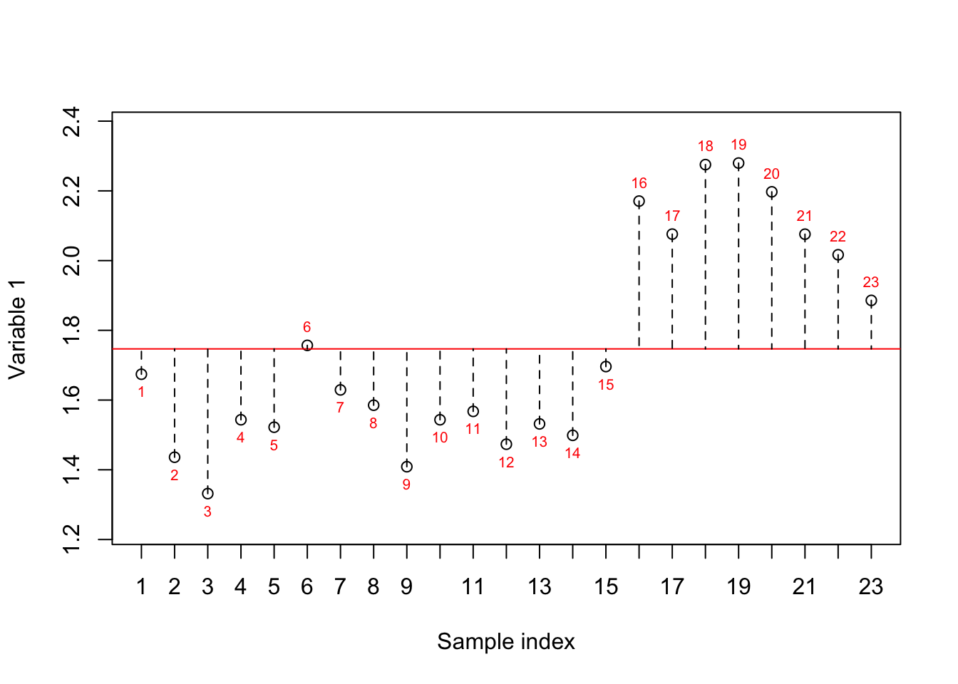
Figure 6.40: Here, we select one variable (a gene) and show how the data is spread around the mean. The red numbers show the index of each sample. The red line shows the mean and the dashed lines show the distance between each observation and mean
This is calculated as \(\sigma^2 = \frac{\sum_{i=1}^{n}(x_i - \mu)^2} {n-1}\) which is saying that for each value in this specific variable, subtract it by the average of the variable and raise it to the power two. Then sum all resulting values and divide the results by \(n-1\). For example if we have \(a=[1,2,3]\), average of \(a\) is \(2\) and the variance is \(\sigma^{2}=\frac{(1-2)^{2}+(2-2)^{2}+(3-2)^{2}}{3-1}=1\)
We also defined covariance as the measure of redundancy in our data. More specifically, if we calculate the covariance between two variables, a value higher than zero means the variable shows similar information in the same direction. If it’s below zero they are showing the opposite information (still redundant but opposite). And if it’s zero, they are showing complementary information.
# define variables
var1<-18924
var2<-20355
# plot the data
plot(data[,c(var1,var2)],xlab = "Variable 1", ylab = "Variable 2")

# fig position of labels
pos_plot<-(as.numeric(sort(data[,variableIndex])>mean(data[,variableIndex]))*2)+1
# Draw sample index
text((data[,var1]), (data[,var2]),  1:nrow(data),
     cex=0.65,pos=pos_plot)

# plot mean of variable 1
abline(v=mean(data[,var1]),col="purple",lty=1)

# plot mean of variable 2
abline(h=mean(data[,var2]),col="coral",lty=1)

for(i in 1:nrow(data))
{

    segments(x0 = (data[,var1])[i],x1 = mean(data[,var1]),y0 = (data[,var2])[i],y1 =  (data[,var2])[i],lty="dashed",
             col=ifelse(data[i,var1]>mean(data[,var1]),yes = "indianred1",no = "lightblue"))


    segments(x0 = (data[,var1])[i],x1 = (data[,var1])[i],y0 = (data[,var2])[i],y1 =  mean(data[,var2]),lty="dashed",
             col=ifelse(data[i,var2]>mean(data[,var2]),yes = "indianred1",no = "lightblue"))
}

# add areas to the plot

text(4,8,"Area 1")
text(10,8,"Area 2")
text(10,2.5,"Area 3")
text(4,2.5,"Area 4")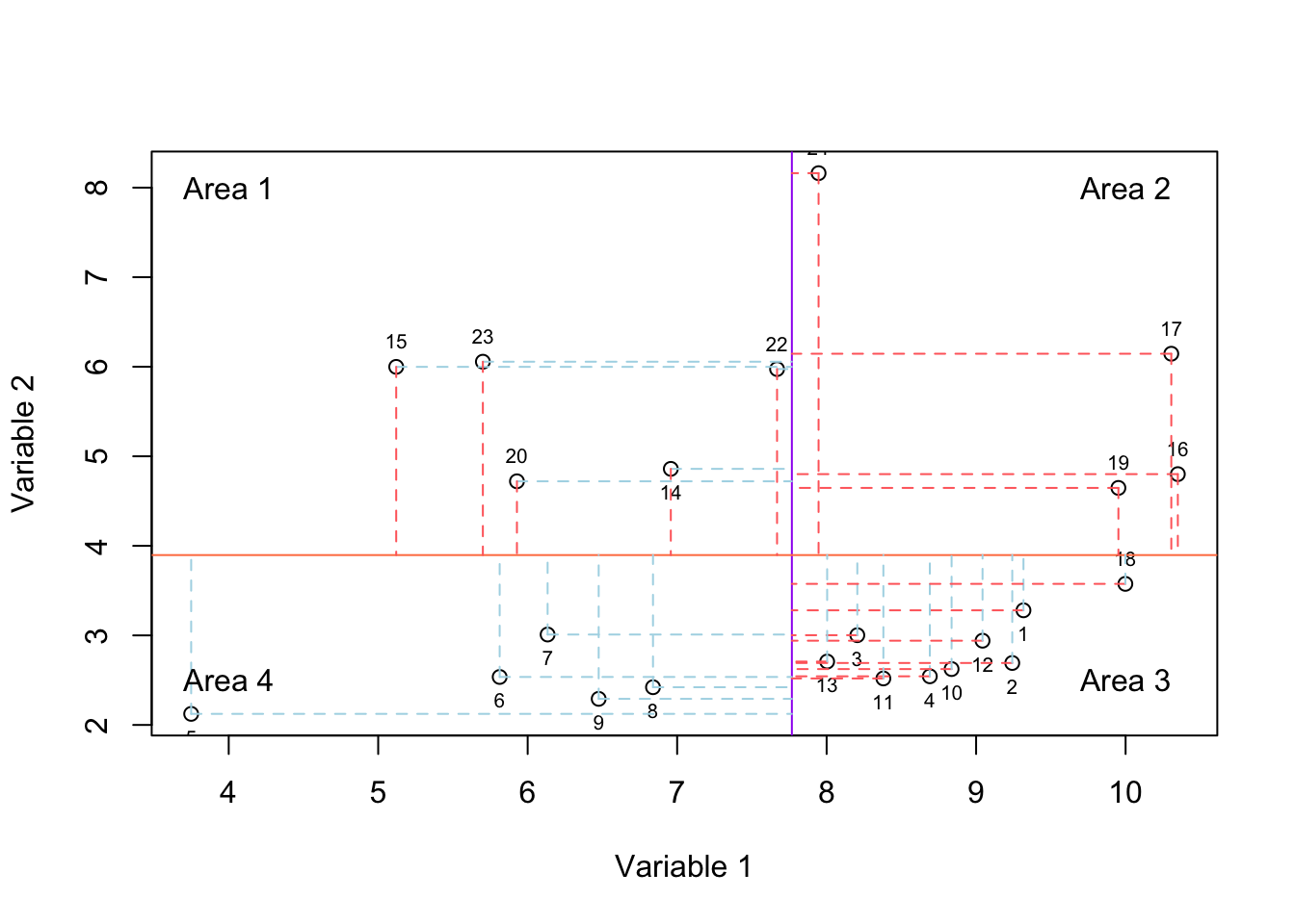
Figure 6.41: Here, we select two variables and show how the data is spread according to both of the variables. The solid purple and coral lines show mean of variable and variable 2, respectively. For each observation, we have two lines showing whether it has higher or lower value compared to mean of variable one and variable 2.
We calculate covariance as \(Cov(x,y)=\frac{\sum_{i=1}^{N}(x_{i}-\bar{x})(y_{i}-\bar{y})}{n-1}\) which is saying (as depicted in Figure 6.41): We have two variables, select the first value in the first variable, find how much it’s going up or down compare to its mean. Now select the corresponding value in the second variable and do the same thing. Multiply the result. Then Do the same thing for all the values in the two variables. Sum the results and divide by number of values. The whole thing is asking where the values of two variables are consistently going up or down compared to their means. For example if we have \(a=[1,2,3]\) and \(b=[4,2,5]\) the covariance of \(a\) with average of \(2\) and \(b\) with average of \(3.6\) is \(Cov(a,b)=\frac{(1-2) \times (4-3.6) + (2-2) \times (2-3.6) + (3-2) \times (5-3.6)}{3-1}=0.5\).
There is a small little thing here! That we often have many variables (thousands) and we have to calculate variance for each of them and covariance for all the two pairs of variables. Can we store this information somewhere? That is a covariance matrix. The diagonal elements in the covariance matrix show variance and the off-diagonal elements show covariance. For example, if we have three variables (three genes): \(a\), \(b\), \(c\), we can define the covariance matrix as follow
\[\begin{array}{c c} & \begin{array}{c c c} a & b &c \\ \end{array} \\ \begin{array}{c c c} a \\ b\\ c \end{array} & \left| \begin{array}{c c c} 0.4 & .3 & 0 \\ 0.3 & 2 & 5 \\ 0 & 5 & 0.8 \end{array} \right| \end{array}\]
We can calculate the covariance matrix of \(A\) simply by doing \(Cov(A)=\frac{1}{n-1} \times A^T \ A\) (look the matrix multiplication). Look at covariance formula, the first part of \(Cov(A)=\frac{1}{n-1} \times A^T \ A\) is \(\frac{1}{n-1}\) which is basically the division we do in \(Cov(x,y)=\frac{\sum_{i=1}^{N}(x_{i}-\bar{x})(y_{i}-\bar{y})}{n-1}\). The second part is doing \(Cov(x,y)=\sum_{i=1}^{N}(x_{i})(y_{i})\) we are missing something! What is that? Subtraction by the average. Here comes the trick. If we center our data, the average of each variable becomes zero. So \(Cov(x,y)=\frac{\sum_{i=1}^{N}(x_{i}-\bar{x})(y_{i}-\bar{y})}{n-1}\) becomes \(Cov(x,y)=\frac{\sum_{i=1}^{N}(x_{i}-0)(y_{i}-0)}{n-1}\) that is exactly \(Cov(A)=\frac{1}{n-1} \times A^T \ A\). There are some functions, software that do covaraince matrix using the tradition formula however, to be safe, make sure that you ALWAYS center your data. In the rest of this chapter, we assume that we have centered our data.
The variance of variable a is 0.4 (diagonal element), the variance of b is 2, and the variance of c is 0.8. The covariance between a and b is 0.3 as defined by the first row and the second column of the matrix or the first column and the second row of the matrix (yes, it’s symmetric! Amazing!). The covariance of b and c is 5 (second row and third column) and so forth. I guess by now you realized we summarized the whole structure of our data is a covariance matrix. It shows how individual variables are spread and how they are related. Well, this pretty much our data characteristics! As we said we like our data to have good variance but low covariance, meaning that we have not wasted our time and money measuring things that show the same thing! But we rather have complementary information. With this definition, what is a nice covariance matrix? It’s a matrix that has zero on the off-diagonal elements (no covariance between any variable in our data) and large numbers on the diagonal elements. Or at least the first one is the largest then the second one and so on. Did I say there is a method (diagonalization) that can take a square matrix and make everything off-diagonal zero and still keep the structure? Yes! We want to apply diagonalization on the covariance matrix to end up with nonzero elements on the diagonal and zero elements elsewhere. This means a structure that is guaranteed to no have redundant information! Awesome! Let’s move on to how we calculate it.
6.4.8 Eigendecomposition of a covariance matrix
There are many methods for diagonalization but here we focus on the classic one using eigendecomposition.
Let’s say our data is sitting in matrix \(X\), in which the rows are observations and the columns are variables. Our goal is to find an orthonormal matrix \(P\) that when we mapped map our original data \(X\) to another space \(Y\) so that the covariance of \(Y\) becomes diagonal (zero on all off-diagonal elements). So the goal is \(Y=X \ P\) so that \(Cov(Y)=diagonal \ or \ \frac{1}{n}Y^T \ Y=diagonal\).
So as said before we can calculate the covariance of the mapped data (\(Y\)) as \(Cov(Y)= \frac{1}{n}Y \ Y^T\). The covariance of the original data (before transformation) is \(Cov(X)= \frac{1}{n}X^T \ X\) We can try to rewrite this formula like this:
\(Cov(Y)= \frac{1}{n}Y^T \ Y\) Did we say that \(Y=XP\) right? So let’s replace \(Y\) by \(XP\) in right side of \(Cov(Y)= \frac{1}{n}Y^T \ Y\)
\(Cov(Y)= \frac{1}{n} (XP)^T \ (XP)\)
We just expand transpose in \((PX)^T\) and write it like \(X^T P^T\) (note that we have to switch the order to \(PX\) to \(XP\)). Now let’s reorder the division by \(n\) and remove the parenthesis.
\(Cov(Y)= P^T\frac{1}{n}X^T XP\)
Great! Do you see something cool in the middle of the equation? Yes. That is the covariance of the original matrix (\(Cov(X)= \frac{1}{n}X^T \ X\)).
\(Cov(Y)= P^T(\frac{1}{n}X^T X)P\)
It reads that if we have to come up with a matrix \(P\) and put it inside a formula, then the covariance of the mapped data becomes diagonal. This is exactly what we wanted! How do we come up with such a matrix \(P\)? There is a theory saying that if we have a symmetric matrix, we can diagonalize it using its eigenvector. What does it mean? We said that we can calculate the covariance matrix of our data and this covariance matrix is symmetric. We can find the eigenvectors of this covariance matrix and use it as \(P\) in \(Cov(Y)= P^T(\frac{1}{n}X^T X)P\). This way we are mapping our data to another space (using eigenvectors) where the mapped data will not have any covariance between its variables. Exactly what we were aiming for. Let’s see a short proof.
Do you remember we have two \(\lambda\) in the eigenvalue section (6.14)? We said that we can put them inside a diagonal matrix like this \(\Lambda= \begin{vmatrix} \lambda & 0 \\ 0 & \lambda \end{vmatrix}\). Doing so our eigenvector formula becomes \(A \ V = \Lambda \ V\) where \(\Lambda\) is a matrix. We said the we want to find eigenvalues for covariance matrix so for (\(Cov(X)\)). So let’s fix the eigen formula first.
\(A \ V = \Lambda \ V\).
How can we make \(Cov(X)\) isolated (separated) from \(V\)? Well, we can multiply both side of the equation with \(V^{-1}\). So our equation become \(Cov(X)=V^{-1} \Lambda \ V\). Maybe we don’t remember anymore, but we said the if we find the eigenvectors of a symmetric matrix, the eigenvectors are orthogonal. There is a super amazing thing about orthogonality. If all the vectors inside a matrix are orthogonal, the inverse of that matrix is equal to its transpose. So we said vectors in \(V\) (containing eigenvectors) are orthogonal, this means \(V^{-1}=V^T\). So let’s fix the equation above:
\(Cov(X)=V \Lambda \ V^T\).
We said that \(Cov(X)=\frac{1}{n}X^TX\) so then \(Cov(X)=V \Lambda \ V^T\) becomes \(\frac{1}{n}XX^T=V \Lambda \ V^T\)
Now it’s much better. We can find covariance of our original data by using the eigenvector and eigenvalues of the covariance matrix. Now let’s get back to the mapped data \(Y\)
\(Cov(Y)= P^T(\frac{1}{n}X^T X)P\)
We said that \(\frac{1}{n}XX^T=V \Lambda \ V^T\) so why not replace \(\frac{1}{n}X^TX\) in \(Cov(Y)= P^T(\frac{1}{n}X^T X)P\) by \(V \Lambda \ V^T\)? Then we get rid of \(X\). Let’s do that
\(Cov(Y)= P^T(V \Lambda \ V^T)P\)
So great! Didn’t we say that one way to diagonalize a symmetric matrix is by its eigenvectors and we said the eigenvectors are in \(P\)? Awesome. We just calculate them. They are in \(V\). Yes!! So Let’s replace \(P\) by \(V\):
\(Cov(Y)= V^T(V \Lambda \ V^T)V\)
We said the \(V^T=V^{-1}\), what is the result of \(V \ V^T\) in this case? It’s an identity matrix or to oversimplify it, it is \(1\).
So, let’s take off the parenthesis and start removing all the \(VV^T\)
\(Cov(Y)= V^TV \Lambda \ V^TV=\Lambda\)
What happened? Well, if we calculate the eigenvalues and eigenvectors of a covariance matrix, then map the data using the eigenvectors, then take the covariance of all the variables in the mapped data, the result will be equal to our eigenvalue matrix. Yes, eigenvalue matrix (\(\Lambda\)) is diagonal, showing that we will NOT have any redundancy in the mapped space. And each eigenvalue (the value on the diagonal of \(\Lambda\)) is the variance of the each variable in the new space! Do you remember we said that eigenvalue show how much space has been changed related to each eigenvector? They are essentially the variance of your new variables. So for application, you start with the eigenvector that has the largest eigenvalue and then move to the second one. That corresponds to taking the PC1, PC2 PC3, etc in PCA.
We are almost reaching the end of this section. Let’s try to summarize what PCA does.
- Take the dataset (gene expression), \(A\)
- Calculate covariance matrix of \(A\) that is \(Cov(A)\)
- Find eigenvectors of \(Cov(A)\), that are \(V\) and eigenvalues of \(Cov(A)\) that are \(\Lambda\)
- Sort the eigenvectors with respect to eigenvalues so the vector with the largest eigenvalue comes first and the second largest come next and so on (the columns of \(V\) are ordered based on \(\Lambda\))
- Multiply \(A\) by sorted \(V\) and call it \(Y\) that is \(Y=A \ v\)
- \(Y\) contains your data in new space (called PC/components/scores)
- Your variables in the new space are NOT correlated
- \(\Lambda\) is the covariance matrix of your new data
- The eigenvalues can also be interpreted as weights PCA has given to your original variables
- The maximum number of eigenvectors is the rank of your data!
Now you can start interpreting PCA! But before saying goodbye. There are a few things I want to mention quickly.
6.5 Extra topics
6.5.1 PCA and ellipses
I understand that the math behind PCA might be too difficult for some people. Probably the best way of understanding what is happening is by showing ellipses.
PCA can be thought of as fitting your data inside an ellipse in 2d (or ellipsoid in n dimensions) then rotating the ellipse so that the axis of the ellipse is aligned with the standard basis.
Let’s look at an example:
par(mfrow=c(1,2))
# define variables
var1<-18924
var2<-20355
var3<-18505

# dfine data
x<-scale(data[,c(var1,var3)],scale = F)
# plot the data
plot(x,xlab = "Variable 1", ylab = "Variable 2",xlim=c(-4,4),ylim=c(-4,4),axes = T)

title("Original data")
# Draw ellipses
heplots:::covEllipses.data.frame(as.data.frame(x),add=T)

# Do PCA
eigen_vectors<-prcomp(x)$rotation

# Draw main axis of ellipses
arrows(0,0,eigen_vectors[1,1],eigen_vectors[2,1],col="red",length=0.1)
arrows(0,0,eigen_vectors[1,2],eigen_vectors[2,2],col="blue",length=0.1)

# plot PCA
plot(prcomp(x)$x,xlim=c(-4,4),ylim=c(-4,4))
title("PCA")
# Draw ellipse
heplots:::covEllipses(as.data.frame(prcomp(x)$x),add=T)

# Rotate eigen vectors
eg2<-eigen_vectors%*%eigen_vectors

# plot arrows
arrows(0,0,eg2[1,1],eg2[2,1],col="red",length=0.1)
arrows(0,0,eg2[1,2],eg2[2,2],col="blue",length=0.1)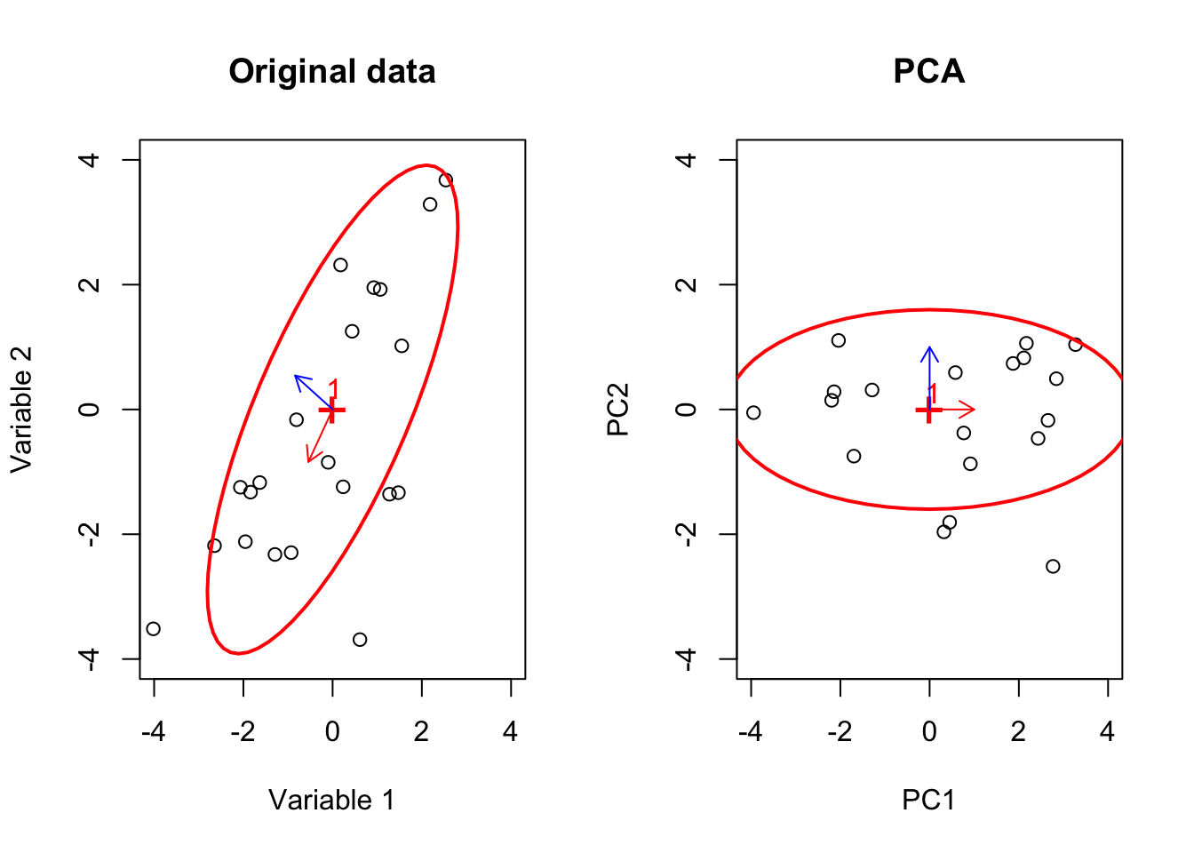
Figure 6.42: Here, we select two variables and show how the data is spread according to both of the variables. We plotted the main axis of the ellipse and showed how it is rotated by PCA
We see that in Figure 6.42, that PCA put an ellipse on the data (the left panel). It finds its main axes The axis are eigenvectors! The axis of the largest spread of the ellipse is the eigenvector with the largest eigenvalue (red arrows) and the second one is the next largest. It then rotates the ellipse around the center so that the eigenvectors are aligned with standard bases \([1,0]\) and \([0,1]\). I hope that it’s giving a better intuition about what PCA does!
6.5.2 Choosing the number of components
I guess one key parameter to set when doing a PCA is to choose the number of components. This is sometimes an arbitrary choice. You can start with for example 2 and go to whatever number that you like. However their methods for choosing the number of components.
For example, one can compute all the components and their eigenvalues. Then we average all the eigenvalues and select those components that have larger eigenvalue than the average. For example for matrix \(A\)
\[Select \ v \ \ if \ \lambda_v > \frac{\sum_{n=1}^{rank(A)}diag(v)}{rank(A)}\]
There are other more iterative methods. For example, doing bootstrapping on the dataset (randomly shuffle the data) and choose the number of components at long as \(\lambda\) in the original dataset is larger than \(\lambda\) in the bootstrapped data.
However, in practice, one might one to try a few first components. If you see a pattern of interest in the first component, there is normally little reason to go beyond \(1\) or \(2\) components.
6.5.3 Eigenvectors and regression
You might end up with some resourcing saying that the PCA eigenvectors are coefficients of linear regression. This is in fact true. The values of eigenvectors can be regarded as coefficients of a multiple linear regression which regresses \(Y\) on \(X\). This means if we assume that our first component is \(Y_{*,1}\), our original data is sitting in \(X\) (with \(n\) variables) and our eigenvector for the first component is \(v=[v_1,v_2,v_3,...,v_n]\), it can be shown that:
\[Y_{*,1}=incetcept+ v_1 \times X_{*,1}+ v_2 \times X_{*,2}+...+v_n \times X_{*,n}+\epsilon\] So the values of eigenvectors can be thought of as the weights our coefficients of a linear model regression PCA scores on original variables.
6.5.4 Eigenvectors, loadings, and correlation
If you remember, we said that the eigenvectors are unit scaled (divided by their magnitude) and are showing the direction of the largest variance. Wouldn’t it be nice to add a little bit more information about the variance of the direction that eigenvectors point to? We can do this by multiplying eigenvectors by the standard deviation of the components. So now they are not only showing the direction but they are also showing the magnitude of importance. If we do that we start seeing some really cool things:
If we scale and center our data so the mean of each variable is zero and its standard deviation is \(1\). The PCA loadings will be equal to the Pearson correlation between the original data and the PC scores.
Recall, the formula for covariance. That is \(Cov(X)=\frac{1}{n-1}X^TX\), The Pearson correlation is given by the covariance divided by pooled standard deviation so. For two variables, we can say \(r=\frac{Cov(x,y)}{\sigma_x \sigma_y}\). In this formula \(\sigma\) is standard deviation of a variable such as \(x\) or \(y\). We already said that we scalled our data so \(\sigma=1\) therefore \(r_{x,y}=\frac{Cov(x,y)}{\sigma_x \sigma_y}==\frac{Cov(x,y)}{1}=Cov(x,y)\). So if we scale our data we can find the correlation matrix between original data \(X\) and PC scores \(Y\) as \(Cov(X,Y)=\frac{1}{n-1}X^TY\)
\[Cov(X,Y)=\frac{1}{n-1}X^TY=\frac{1}{n-1}(YV^T)^TY=\frac{1}{n-1}VY^TY =V\frac{1}{n-1}Y^TY \] Didn’t we say that the covariance of Y is \(Cov(Y)= \frac{1}{n-1}Y^TY= V^TV \Lambda \ V^TV=\Lambda\) So then we replace \[Cov(X,Y)=V\frac{1}{n-1}Y^TY=V \Lambda \] This is basically saying that if we scale our eigenvectors by eigenvalues we then have covariance between the original data \(X\) and PCA scores \(Y\). If we take the square root of \(\Lambda\) we have the correlation, only and only if we have scaled our data.
\(r(X,Y)=V\sqrt{\Lambda}\)
This will come in handy when you start interpreting the results.
6.5.5 Eigenvector decomposition vs. singular value decomposition
As said, eigenvector decomposition is only valid on square matrices. We data is normally not square. In PCA, we are interested in variance so PCA does a trick and converts our data to the square form by just taking covariance matrix. It then does eigenvector decomposition on the covariance matrix to diagonalize the covariance matrix giving us only variance.
Calculating the covariance matrix for a large dataset is computationally difficult. We will need to calculate all possible pairwise combinations of all variables which might take a lot of time and memory. In addition, some people might not want to do PCA. They might want to decompose their matrix which is not necessarily a square matrix.
People came up with a solution that can do decomposition on any matrix (necessary a square matrix). This method is called singular value decomposition or SVD. The very detail of this method is well beyond this scope of this chapter but we can quickly have a look at it.
Singular value decomposition says that I can decompose any matrix \(X\) to \(X=USV^T\). In this case, \(V^T\) has all the eigenvectors, \(S\) is all the eigenvalues and \(US\) is all the PC scores. Remember, \(U\) and \(V\) are both orthonormal matrices. Isn’t this cool? If we have a matrix \(X\) and its eigenvectors \(V\), we can diagonalize it, exactly like we did in eigenvector decomposition. However, in PCA we are not interested in diagonalizing \(X\) but we want to do it for the covariance matrix. How do we solve this?
One traditional way to solve \(X=USV^T\) is to multiply it by itself (transpose) and solve it like eigenvector decomposition:
\(X=USV^T\)
\(X^T=VS^TU^T\)
\(X^TX=VS^TU^T \ USV^T\)
We know that if \(U\) and \(V\) are orthonormal, then \(UU^T=U^TU=I\) and \(VV^T=V^TV=I\). In addition, \(S\) is diagonal so \(S=S^T\) meaning that we can simplify the above equation to
\(X^TX=VS^TU^T \ USV^T=VS^2V^T\)
Bringing \(V^T\) to the other side will give us \(X^TXV=VS^2\) What is this? If you remember this looks like the eigenvector decomposition formula:
\[A \ V = \Lambda \ V\] With this difference that \(A=X^TX\). We can solve this and we get to the same results.
In practice, you saw that this approach did not change our computational problem. In fact, SVD is nowadays calculated using iterative methods that will almost never calculate the whole covariance matrix, letting us do PCA for very large datasets.
6.5.6 Assumptions of PCA
PCA like any other method has some assumptions about the data and space. Here are some of the most important ones
PCA assumes a multivariate normal distribution. As you saw for the ellipsoid example, elliptical distribution is just the generalization of normal distribution. You should also make sure that variance and covariance have meaning in your distribution. I would like to mention that, your data does not need to be strictly normally distributed. PCA works with moderately skewed data. However, if your data is very different from the normal distribution, you will have a problem with PCA
I guess you realized that PCA work by doing the linear transformation. This means if you suspect a non-linear relationship between your variables, PCA will be probably not that suitable
When doing PCA, our interest in variance between the observations. If your interest is not variance, PCA is not the method of choice
6.6 Final notes
Thanks for reading this chapter. I know the math behind PCA or any other method can be complicated. It’s not required to know the math to be able to apply PCA to your data. It’s just important that you understand the key concept and the thing that PCA does for you. Please remember now, PCA is just a tool. It does not replace a statistician. If for example, the assumptions are not met, this does not invalidate the method itself but it might change the meaning of the results leading to false interpretations. Please go ahead and apply the method to your data but it’s always a good idea to discuss your results with your statistician before concluding anything about the experiment.
Have fun!